Create a Bitcoin trading robot that won’t lose money

Let’s use reinforcement learning in AI to build a digital currency trading robot.

In this article, we will create and apply an enhanced learning frame number to learn how to make a Bitcoin trading robot. In this tutorial, we will use the gym of OpenAI and the PPO robot from the stable-baselines library, which is a branch of the OpenAI baseline library.

Thank you very much for the open source software provided by OpenAI and DeepMind for the researchers of deep learning in the past few years. If you haven’t seen their amazing achievements with AlphaGo, OpenAI Five, AlphaStar and other technologies, you may have been living in isolation last year, but you should check them out.

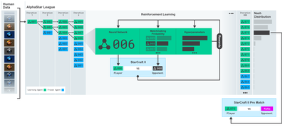
AlphaStar training: https://deepmind.com/blog/alphastar-mastering-real-time-strategy-game-starcraft-ii/

Although we will not create anything impressive, it is still not easy to trade Bitcoin robots in daily transactions. However, as Teddy Roosevelt once said,

There is no value in anything that is too simple.

Therefore, not only should we learn to trade ourselves, but also let robots trade for us.

Plan

1. Create a gym environment for our robot to perform machine learning

2. Render a simple and elegant visual environment

3. Train our robot to learn a profitable trading strategy

If you are not familiar with how to create gym environments from scratch, or how to simply render the visualization of these environments. Before continuing, please feel free to google an article of this kind. These two actions will not be difficult for even the most junior programmers.

Getting Started

In this tutorial, we will use the Kaggle dataset generated by Zielak. If you want to download the source code, it will be provided in my Github repository, along with the .csv data file. Ok, let’s start.

First, let’s import all the necessary libraries. Make sure to use pip to install any libraries you are missing.

import gym
import pandas as pd
import numpy as np
from gym import spaces
from sklearn import preprocessing

Next, let’s create our class for the environment. We need to pass in a Pandas data frame number and an optional initial_balance and a lookback_indow_size, which will indicate the number of past time steps observed by the robot in each step. We default the commission of each transaction to 0.075%, that is, the current exchange rate of Bitmex, and default the serial parameter to false, which means that our data frame number will be traversed by random fragments by default.

We also call dropna() and reset_index() on the data, first delete the row with NaN value, and then reset the index of frame number, because we have deleted the data.

class BitcoinTradingEnv(gym.Env):
  """A Bitcoin trading environment for OpenAI gym"""
  metadata = {'render.modes': ['live', 'file', 'none']}
  scaler = preprocessing.MinMaxScaler()
  viewer = None
def __init__(self, df, lookback_window_size=50, 
                         commission=0.00075,  
                         initial_balance=10000
                         serial=False):
    super(BitcoinTradingEnv, self).__init__()
self.df = df.dropna().reset_index()
    self.lookback_window_size = lookback_window_size
    self.initial_balance = initial_balance
    self.commission = commission
    self.serial = serial
# Actions of the format Buy 1/10, Sell 3/10, Hold, etc.
    self.action_space = spaces.MultiDiscrete([3, 10])
# Observes the OHCLV values, net worth, and trade history
    self.observation_space = spaces.Box(low=0, high=1, shape=(10, lookback_window_size + 1), dtype=np.float16)

Our action_space is represented as a group of 3 options (buy, sell or hold) here and another group of 10 amounts (1/10, 2/10, 3/10, etc.). When we choose to buy, we will buy amount * self.balance word of BTC. For selling, we will sell amount * self.btc_held worth of BTC. Of course, holding will ignore the amount and do nothing.

Our observation_space is defined as a continuous floating point set between 0 and 1, and its shape is (10, lookback_window_size+1). + 1 is used to calculate the current time step. For each time step in the window, we will observe the OHCLV value. Our net worth is equal to the number of BTCs we buy or sell, and the total amount of dollars we spend or receive on these BTCs.

Next, we need to write the reset method to initialize the environment.

def reset(self):
  self.balance = self.initial_balance
  self.net_worth = self.initial_balance
  self.btc_held = 0
self._reset_session()
self.account_history = np.repeat([
    [self.net_worth],
    [0],
    [0],
    [0],
    [0]
  ], self.lookback_window_size + 1, axis=1)
self.trades = []
return self._next_observation()

Here we use self._reset_session and self._next_observation, which we haven’t defined yet. Let’s define them first.

Trade session

An important part of our environment is the concept of trading sessions. If we deploy this robot outside the market, we may never run it for more than a few months at a time. For this reason, we will limit the number of consecutive frames in self.df, which is the number of frames that our robot can see at one time.

In our _reset_session method, we reset the current_step to 0 first. Next, we will set steps_left to a random number between 1 to MAX_TRADING_SESSIONS, which we will define at the top of the program.

MAX_TRADING_SESSION = 100000 ＃ ~2 months

Next, if we want to traverse the number of frames consecutively, we must set it to traverse the entire number of frames, otherwise we set frame_start to a random point in self.df and create a new data frame named active_df, which is just a slice of self.df and it’s getting from frame_start to frame_start + steps_left.

def _reset_session(self):
  self.current_step = 0
if self.serial:
    self.steps_left = len(self.df) - self.lookback_window_size - 1
    self.frame_start = self.lookback_window_size
  else:
    self.steps_left = np.random.randint(1, MAX_TRADING_SESSION)
    self.frame_start = np.random.randint(self.lookback_window_size, len(self.df) - self.steps_left)
self.active_df = self.df[self.frame_start - self.lookback_window_size:self.frame_start + self.steps_left]

An important side effect of traversing the number of data frames in the random slice is that our robot will have more unique data for use in long-term training. For example, if we only traverse the number of data frames in a serial way (that is, from 0 to len(df)), we will only have as many unique data points as the number of data frames. Our observation space can only use a discrete number of states at each time step.

However, by traversing the slices of the data set randomly, we can create a more meaningful set of trading results for each time step in the initial data set, that is, the combination of trading behavior and price behavior seen previously to create more unique data sets. Let me give an example to explain.

When the time step after resetting the serial environment is 10, our robot will always run in the data set at the same time, and there are three options after each time step: buy, sell or hold. For each of the three options, you need another option: 10%, 20%, … or 100% of the specific implementation amount. This means that our robot may encounter one of the 10 states of any 103, a total of 1030 cases.

Now back to our random slicing environment. When the time step is 10, our robot may be in any len(df) time step within the number of data frames. Assuming that the same choice is made after each time step, it means that the robot can experience the unique state of any len(df) to the 30th power in the same 10 time steps.

Although this may bring considerable noise to large data sets, I believe that robots should be allowed to learn more from our limited data. We will still traverse our test data in a serial way to obtain the freshest and seemingly ‘real-time’ data, in order to obtain a more accurate understanding through the effectiveness of the algorithm.

Observed through the eyes of a robot

Through effective visual environment observation, it is often helpful to understand the type of functions that our robot will use. For example, here is the visualization of observable space rendered using OpenCV.

Observation of OpenCV visualization environment

Each line in the image represents a row in our observation_space. The first four lines of red lines with similar frequencies represent OHCL data, and the orange and yellow dots directly below represent trading volume. The fluctuating blue bar below represents the net value of the robot, while the lighter bar below represents the transaction of the robot.

If you observe carefully, you can even make a candle map yourself. Below the trading volume bar is a Morse code interface, displaying the trading history. It seems that our robot should be able to learn sufficiently from the data in our observation_space, so let’s continue. Here, we will define the _next_observation method, we scale the observed data from 0 to 1.

• It is important to extend only the data observed by the robot so far to prevent leading deviation.

def _next_observation(self):
  end = self.current_step + self.lookback_window_size + 1
obs = np.array([
    self.active_df['Open'].values[self.current_step:end],  
    self.active_df['High'].values[self.current_step:end],
    self.active_df['Low'].values[self.current_step:end],
    self.active_df['Close'].values[self.current_step:end],
    self.active_df['Volume_(BTC)'].values[self.current_step:end],])
scaled_history = self.scaler.fit_transform(self.account_history)
obs = np.append(obs, scaled_history[:, -(self.lookback_window_size + 1):], axis=0)
return obs

Take action

We have established our observation space, and now it is time to write our ladder function, and then take the robot’s scheduled action. Whenever self.steps_left == 0 for our current trading session, we will sell our BTC and call _reset_session(). Otherwise, we will set reward to the current net value. If we run out of funds, we will set done to True.

def step(self, action):
  current_price = self._get_current_price() + 0.01
  self._take_action(action, current_price)
  self.steps_left -= 1
  self.current_step += 1
if self.steps_left == 0:
    self.balance += self.btc_held * current_price
    self.btc_held = 0
    self._reset_session()
obs = self._next_observation()
  reward = self.net_worth
  done = self.net_worth <= 0
return obs, reward, done, {}

Taking trading action is as simple as getting current_price, determining the actions to be executed and the quantity to buy or sell. Let’s quickly write _take_action so that we can test our environment.

def _take_action(self, action, current_price):
  action_type = action[0]
  amount = action[1] / 10
btc_bought = 0
  btc_sold = 0
  cost = 0
  sales = 0
if action_type < 1:
    btc_bought = self.balance / current_price * amount
    cost = btc_bought * current_price * (1 + self.commission)
    self.btc_held += btc_bought
    self.balance -= cost
elif action_type < 2:
    btc_sold = self.btc_held * amount
    sales = btc_sold * current_price  * (1 - self.commission)
    self.btc_held -= btc_sold
    self.balance += sales

Finally, in the same method, we will attach the transaction to self.trades and update our net value and account history.

if btc_sold > 0 or btc_bought > 0:
    self.trades.append({
      'step': self.frame_start+self.current_step,
      'amount': btc_sold if btc_sold > 0 else btc_bought,
      'total': sales if btc_sold > 0 else cost,
      'type': "sell" if btc_sold > 0 else "buy"
    })
self.net_worth = self.balance + self.btc_held * current_price
  self.account_history = np.append(self.account_history, [
    [self.net_worth],
    [btc_bought],
    [cost],
    [btc_sold],
    [sales]
  ], axis=1)

Our robot can start a new environment now, complete the environment gradually, and take actions that affect the environment. It’s time to watch the trade.

Watch our robot trade

Our rendering method can be as simple as calling print (self.net_word), but it is not interesting enough. Instead, we will draw a simple candle chart, which contains a separate chart of the trading volume column and our net worth.

We will get the code in StockTrackingGraph.py from my last article and redesign it to adapt to the Bitcoin environment. You can get the code from my Github.

The first change we need to make is to update self.df ['Date '] to self.df [‘Timestamp’] and delete all calls to date2num, because our date is already in unix timestamp format. Next, in our rendering method, we will update the date tag to print human-readable dates instead of numbers.

from datetime import datetime

First, import the datetime library, and then we will use utcfromtimestampmethod to obtain the UTC string from each timestamp and strftime so that it is formatted as a string: Y-m-d H:M format.

date_labels = np.array([datetime.utcfromtimestamp(x).strftime('%Y-%m-%d %H:%M') for x in self.df['Timestamp'].values[step_range]])

Finally, we will change self. df['Volume '] to self. df[‘Volume_ (BTC)’] to match our dataset. After completing these, we are ready. Back to our BitcoinTradingEnv, we can write rendering methods to display the chart now.

def render(self, mode='human', **kwargs):
  if mode == 'human':
    if self.viewer == None:
      self.viewer = BitcoinTradingGraph(self.df,
                                        kwargs.get('title', None))
self.viewer.render(self.frame_start + self.current_step,
                       self.net_worth,
                       self.trades,
                       window_size=self.lookback_window_size)

We can watch our robots trade Bitcoin now.

Visualize our robot trading with Matplotlib

The green phantom label represents the buying of BTC, and the red phantom label represents the selling. The white label in the upper right corner is the current net value of the robot, and the label in the lower right corner is the current price of Bitcoin. It’s simple and elegant. Now, it’s time to train our robots and see how much money we can make!

Training time

One of the criticisms I received in the previous article was lack of cross-validation and the failure to divide the data into training sets and test sets. The purpose of this is to test the accuracy of the final model on new data that has never been seen before. Although this is not the focus of that article, it is really very important. Because we use time series data, we don’t have many choices in cross validation.

For example, a common form of cross-validation is called k-fold validation. In this validation, you divide the data into k equal groups, one by one, individually, as the test group and use the rest of the data as the training group. However, time series data are highly dependent on time, which means that subsequent data is highly dependent on previous data. So k-fold will not work, because our robot will learn from future data before trading, which is an unfair advantage.

When applied to time series data, the same flaw applies to most other cross-validation strategies. Therefore, we only need to use a part of the complete data frame number as the training set from the frame number to some arbitrary indexes, and use the rest of the data as the test set.

slice_point = int(len(df) - 100000)
train_df = df[:slice_point]
test_df = df[slice_point:]

Next, since our environment is only set up to handle a single number of data frames, we will create two environments, one for the training data and one for the test data.

train_env = DummyVecEnv([lambda: BitcoinTradingEnv(train_df, commission=0, serial=False)])
test_env = DummyVecEnv([lambda: BitcoinTradingEnv(test_df, commission=0, serial=True)])

Now, training our model is as simple as creating a robot using our environment and calling model.learn.

model = PPO2(MlpPolicy,
             train_env,
             verbose=1, 
             tensorboard_log="./tensorboard/")
model.learn(total_timesteps=50000)

Here, we use tensor plates, so we can visualize our tensor flow charts easily and view some quantitative indicators about our robot. For example, the following is the discounted rewards chart of many robots with more than 200,000 time steps:

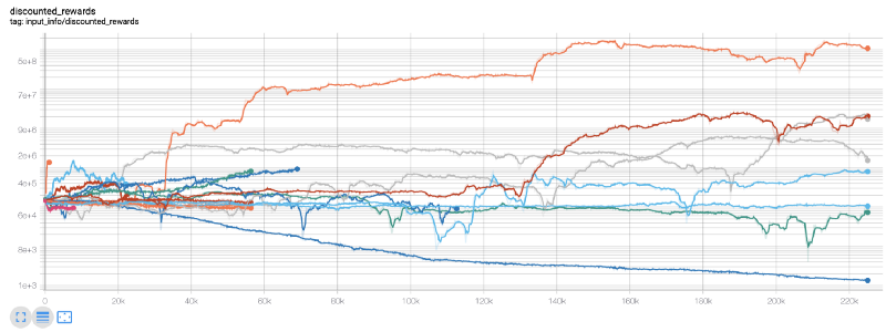
Wow, it seems that our robot is very profitable! Our best robot can even achieve 1000x balance in 200,000 steps, and the rest will increase at least 30 times on average!

At this time, I realized that there was a mistake in the environment… After fixing the bug, this is the new reward chart:

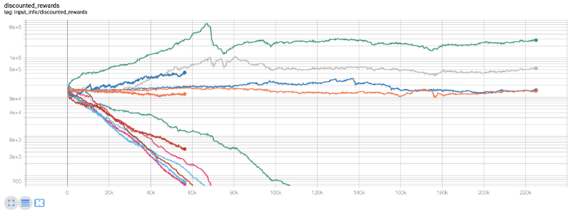
As you can see, some of our robots are doing well, while others are going bankrupt. However, robots with good performance can reach 10 times or even 60 times the initial balance at most. I must admit that all profitable machines are trained and tested without commission, so it is unrealistic for our robots to make any real money. But at least we found the way!

Let’s test our robots in the test environment (using new data they have never seen before) to see how they will behave.

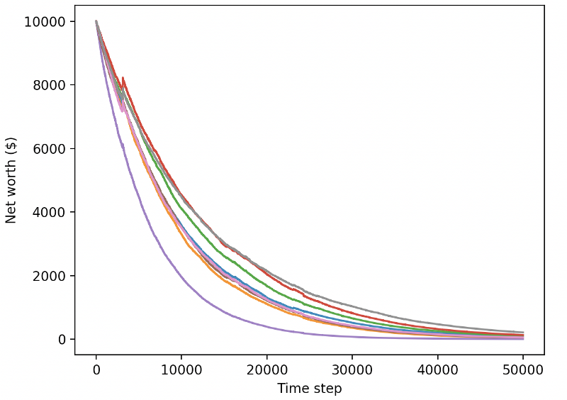
Our well-trained robots will go bankrupt when trading new test data

Obviously, we still have a lot of work to do. By simply switching models to use A2C with stable baseline instead of the current PPO2 robot, we can improve our performance on this data set greatly. Finally, according to Sean O’Gorman’s suggestion, we can update our reward function slightly, so that we can add reward to net worth, rather than just realize high net worth and stay there.

reward = self.net_worth - prev_net_worth

These two changes alone can improve the performance of the test dataset greatly, and as you can see below, we were finally able to profit on new data that were not available in the training set.

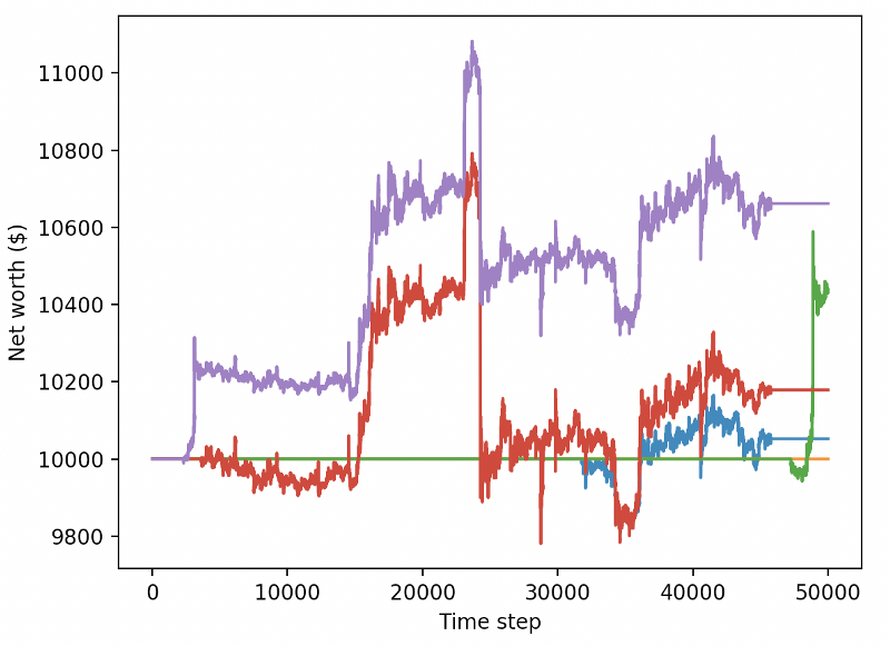
But we can do better. In order to improve these results, we need to optimize our super parameters and train our robots for a longer time. It’s time for the GPU to start working and firing on all cylinders!

So far, this article has been a little long, and we still have many details to consider, so we plan to take a rest here. In the next article, we will use Bayesian optimization to partition the best hyperparameters for our problem space and prepare for training/testing on GPU using CUDA.

Conclusion

In this article, we begin to use reinforcement learning to create a profitable Bitcoin trading robot from scratch. We can complete the following tasks:

1. Create a Bitcoin trading environment from scratch using OpenAI’s gym.

2. Use Matplotlib to build the visualization of the environment.

3. Use simple cross-validation to train and test our robot.

4. Adjust our robots slightly to achieve profits.

Although our trading robot was not as profitable as we had hoped, we are already moving in the right direction. Next time, we will ensure that our robots can consistently beat the market. We will see how our trading robots process real-time data. Please continue to follow my next article and Viva Bitcoin!

Related

More