Thinking about high-frequency trading strategies (3)
Author: The grass, Created: 2023-08-07 18:17:28, Updated: 2023-09-18 19:50:53
In the previous article, I explained how to model cumulative turnover, as well as a simple analysis of price shock phenomena. This article will also continue to analyze the data around trades orders.
Order time intervals
In general, it is assumed that the time of arrival of the order is in line with the Parson process.The Parson ProcessI'll prove it below.
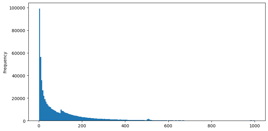
The aggTrades downloaded on August 5, with a total of 193193 trades, is very exaggerated. First of all, look at the distribution of payments, you can see that there is a slippery local peak at around 100ms and 500ms, which should be caused by the robot timing order commissioned by the iceberg, which may also be one of the reasons for the unusual behavior of the day.
The probability mass function (PMF) of the Parsons distribution is given by:
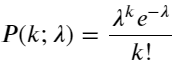
Some of them are:
- k is the number of events we are interested in.
- λ is the average occurrence of events in unit time (or unit space).
- P ((k; λ) denotes the probability of k events occurring by chance under given mean occurrence conditions λ.
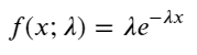
In the Parson process, the time interval between events is subject to an exponential distribution. The probability density function of the exponential distribution (PDF) is given by the formula:
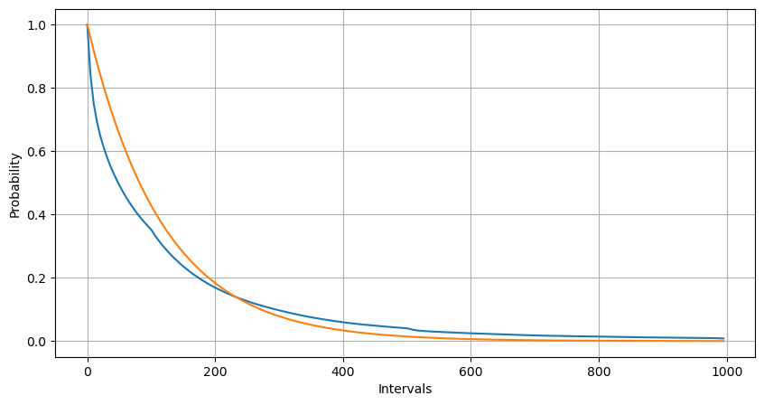
By matching the findings with the expected differences in the Pareto distribution, the Pareto process underestimated the frequency of long interval times and overestimated the frequency of low interval times.
from datetime import date,datetime
import time
import pandas as pd
import numpy as np
import matplotlib.pyplot as plt
%matplotlib inline
trades = pd.read_csv('YGGUSDT-aggTrades-2023-08-05.csv')
trades['date'] = pd.to_datetime(trades['transact_time'], unit='ms')
trades.index = trades['date']
buy_trades = trades[trades['is_buyer_maker']==False].copy()
buy_trades = buy_trades.groupby('transact_time').agg({
    'agg_trade_id': 'last',
    'price': 'last',
    'quantity': 'sum',
    'first_trade_id': 'first',
    'last_trade_id': 'last',
    'is_buyer_maker': 'last',
    'date': 'last',
    'transact_time':'last'
})
buy_trades['interval']=buy_trades['transact_time'] - buy_trades['transact_time'].shift()
buy_trades.index = buy_trades['date']
buy_trades['interval'][buy_trades['interval']<1000].plot.hist(bins=200,figsize=(10, 5));
Intervals = np.array(range(0, 1000, 5))
mean_intervals = buy_trades['interval'].mean()
buy_rates = 1000/mean_intervals
probabilities = np.array([np.mean(buy_trades['interval'] > interval)  for interval in Intervals])
probabilities_s = np.array([np.e**(-buy_rates*interval/1000) for interval in Intervals])

plt.figure(figsize=(10, 5))
plt.plot(Intervals, probabilities)
plt.plot(Intervals, probabilities_s)
plt.xlabel('Intervals')
plt.ylabel('Probability')
plt.grid(True)
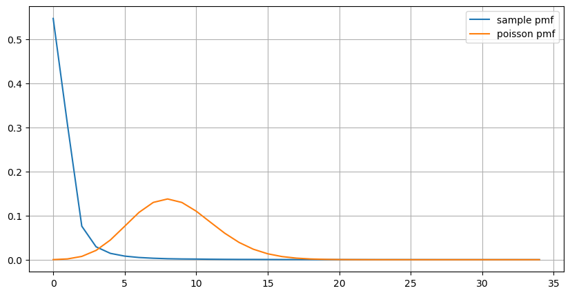
The statistical distribution of the number of times an order occurs in 1s, compared to the Parsons distribution, is also very different. Parsons distribution significantly underestimates the frequency of small probability events.
- Non-constant incidence: The Parsons process assumes that the average incidence of an event in any given time interval is a constant. If this assumption is not true, then the distribution of the data will deviate from the Parsons distribution.
- Interaction of processes: Another basic assumption of Parsons processes is that events are independent of one another. If events in the real world influence one another, then their distribution may deviate from the Parsons distribution.
That is, in a real-world environment, the frequency at which orders occur is non-constant, requires real-time updates, and there is an incentive effect, i.e. more orders in a fixed time will trigger more orders. This makes it impossible for the strategy to fix a single parameter.
result_df = buy_trades.resample('0.1S').agg({
    'price': 'count',
    'quantity': 'sum'
}).rename(columns={'price': 'order_count', 'quantity': 'quantity_sum'})
count_df = result_df['order_count'].value_counts().sort_index()[result_df['order_count'].value_counts()>20]
(count_df/count_df.sum()).plot(figsize=(10,5),grid=True,label='sample pmf');

from scipy.stats import poisson
prob_values = poisson.pmf(count_df.index, 1000/mean_intervals)

plt.plot(count_df.index, prob_values,label='poisson pmf');
plt.legend() ;
Updating parameters in real time
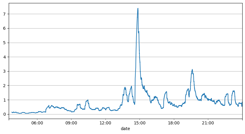
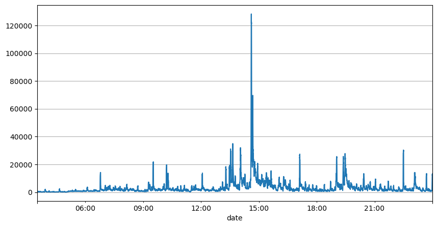
From the above analysis of the order intervals, it can be concluded that the fixed parameters are not suitable for the real market, and the key parameters of the strategy for the market description need to be updated in real time. The easiest solution to think of is the moving average of the sliding window. The following two graphs are the average of the frequency of payments within 1s and the volume of transactions in 1000 windows, respectively.
The graph also shows why the order frequency deviates so much from the Parsons distribution, where the average order number per second is only 8.5 times, but in extreme cases the average order number per second deviates significantly.
Here, it was found that the parallax error was the smallest predicted with the mean of the first two seconds, and far better than simple mean prediction results.
result_df['order_count'][::10].rolling(1000).mean().plot(figsize=(10,5),grid=True);
result_df
| order_count | quantity_sum | |
|---|---|---|
| 2023-08-05 03:30:06.100 | 1 | 76.0 |
| 2023-08-05 03:30:06.200 | 0 | 0.0 |
| 2023-08-05 03:30:06.300 | 0 | 0.0 |
| 2023-08-05 03:30:06.400 | 1 | 416.0 |
| 2023-08-05 03:30:06.500 | 0 | 0.0 |
| … | … | … |
| 2023-08-05 23:59:59.500 | 3 | 9238.0 |
| 2023-08-05 23:59:59.600 | 0 | 0.0 |
| 2023-08-05 23:59:59.700 | 1 | 3981.0 |
| 2023-08-05 23:59:59.800 | 0 | 0.0 |
| 2023-08-05 23:59:59.900 | 2 | 534.0 |
result_df['quantity_sum'].rolling(1000).mean().plot(figsize=(10,5),grid=True);
(result_df['order_count'] - result_df['mean_count'].mean()).abs().mean()
6.985628185332997
result_df['mean_count'] = result_df['order_count'].ewm(alpha=0.11, adjust=False).mean()
(result_df['order_count'] - result_df['mean_count'].shift()).abs().mean()
0.6727616961866929
result_df['mean_quantity'] = result_df['quantity_sum'].ewm(alpha=0.1, adjust=False).mean()
(result_df['quantity_sum'] - result_df['mean_quantity'].shift()).abs().mean()
4180.171479076811
Summary
This article briefly describes the reasons for the order time interval deviation process, mainly because the parameters change over time. To more accurately forecast the market, the strategy requires real-time forecasting of the basic parameters of the market. The remainder can be used to measure the good and bad of the forecast, the simplest example is given above.
- Smiley curve for delta hedging of bitcoin options
- Thoughts on High-Frequency Trading Strategies (5)
- Thoughts on High-Frequency Trading Strategies (4)
- Thinking about high-frequency trading strategies (5)
- Thinking about high-frequency trading strategies (4)
- Thoughts on High-Frequency Trading Strategies (3)
- Thoughts on High-Frequency Trading Strategies (2)
- Thinking about high-frequency trading strategies (2)
- Thoughts on High-Frequency Trading Strategies (1)
- Thinking about high-frequency trading strategies (1)
- Futu Securities Configuration Description Document
- FMZ Quant Uniswap V3 Exchange Pool Liquidity Related Operations Guide (Part 1)
- FMZ Quantitative Uniswap V3 Exchange Pool Liquidity related operating manual (1)