Creating a Bitcoin trading robot that won't lose money

Let's use reinforcement learning in AI to build a digital currency trading robot.

In this article, we will create and apply a reinforcement learning algorithm to learn how to make a Bitcoin trading robot. In this tutorial, we will use OpenAI's gym and PPO robots from the stable-baselines library, a branch of the OpenAI database.

Thank you so much for the open source software that OpenAI and DeepMind have provided to deep learning researchers over the past few years. If you haven't seen their amazing achievements with technologies like AlphaGo, OpenAI Five, and AlphaStar, you may have been living outside of isolation for the past year, but you should check them out.

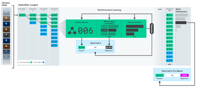
AlphaStar traininghttps://deepmind.com/blog/alphastar-mastering-real-time-strategy-game-starcraft-ii/

While we won't create anything impressive, it's still not easy to trade Bitcoin robots in everyday transactions.

It's not worth anything to get something that's too easy.

So, not only should we learn to trade for ourselves... but also let robots trade for us.

The Plan

1.为我们的机器人创建gym环境以供其进行机器学习

2.渲染一个简单而优雅的可视化环境

3.训练我们的机器人，使其学习一个可获利的交易策略

If you're not familiar with how to create gym environments from scratch, or how to visualise simple renderings of these environments; before continuing, please google an article like this one. These two actions won't be difficult even as a beginner programmer.

The entrance

在本教程中，我们将使用Zielak生成的Kaggle数据集。如果您想下载源代码，我的Github仓库中会提供，同时也有.csv数据文件。好的，让我们开始吧。

First, let's import all the necessary libraries. Make sure to install any libraries you're missing with pip.

import gym
import pandas as pd
import numpy as np
from gym import spaces
from sklearn import preprocessing

Next, let's create our class for the environment. We need to pass a panda's data threshold, as well as an optional initial_balance and a lookback_window_size, which will indicate the past time steps the robot observed in each step. We default to a commission of 0.075% per transaction, i.e. the current exchange rate of Bitmex, and set the string parameter to default to false, which means that by default our data threshold will run through random segments.

We also call the data dropna (() and reset_index ((), first deleting the row with the NaN value, and then resetting the index with the bit count, since we have deleted the data.

class BitcoinTradingEnv(gym.Env):
  """A Bitcoin trading environment for OpenAI gym"""
  metadata = {'render.modes': ['live', 'file', 'none']}
  scaler = preprocessing.MinMaxScaler()
  viewer = None
def __init__(self, df, lookback_window_size=50, 
                         commission=0.00075,  
                         initial_balance=10000
                         serial=False):
    super(BitcoinTradingEnv, self).__init__()
self.df = df.dropna().reset_index()
    self.lookback_window_size = lookback_window_size
    self.initial_balance = initial_balance
    self.commission = commission
    self.serial = serial
# Actions of the format Buy 1/10, Sell 3/10, Hold, etc.
    self.action_space = spaces.MultiDiscrete([3, 10])
# Observes the OHCLV values, net worth, and trade history
    self.observation_space = spaces.Box(low=0, high=1, shape=(10, lookback_window_size + 1), dtype=np.float16)

Our action_space is represented here as a set of 3 options (buy, sell or hold) and another set of 10 amounts (buy 1/10, 2/10, 3/10 etc.). When choosing to buy, we will buy amount * self.balance worth of BTC. For selling, we will sell amount * self.btc_held worth of BTC. Of course, holding will ignore the amount and do nothing.

Our observation_space is defined as a continuous floating-point set between 0 and 1, shaped as ((10, lookback_window_size + 1)); + 1 is used to calculate the current time step. For each time step in the window, we will observe the OHCLV value. Our net worth is equal to the amount of BTC we bought or sold, and the total amount of dollars we spent or received on these BTCs.

Next, we need to write a reset method to initialize the environment.

def reset(self):
  self.balance = self.initial_balance
  self.net_worth = self.initial_balance
  self.btc_held = 0
self._reset_session()
self.account_history = np.repeat([
    [self.net_worth],
    [0],
    [0],
    [0],
    [0]
  ], self.lookback_window_size + 1, axis=1)
self.trades = []
return self._next_observation()

Here we use self._reset_session and self._next_observation, which we haven't defined yet. Let's define them first.

Negotiating

我们环境的一个重要部分是交易会话的概念。如果我们将这个机器人部署到市场外，我们可能永远不会一次运行它超过几个月。出于这个原因，我们将限制self.df中连续帧数的数量，也就是我们的机器人连续一次能看到的帧数。

In our _reset_session method, we first reset the current_step to 0; next, we set the steps_left to a random number between 1 and MAX_TRADING_SESSION, which we define at the top of the program.

MAX_TRADING_SESSION = 100000 ＃ ~2个月

Next, if we want to continuously traverse the array, we have to set it to traverse the entire array, otherwise we set frame_start to a random point in self.df and create a new data array called active_df, which is just a slice of self.df and is derived from frame_start to frame_start + steps_left.

def _reset_session(self):
  self.current_step = 0
if self.serial:
    self.steps_left = len(self.df) - self.lookback_window_size - 1
    self.frame_start = self.lookback_window_size
  else:
    self.steps_left = np.random.randint(1, MAX_TRADING_SESSION)
    self.frame_start = np.random.randint(self.lookback_window_size, len(self.df) - self.steps_left)
self.active_df = self.df[self.frame_start - self.lookback_window_size:self.frame_start + self.steps_left]

An important side-effect of traversing data bits in random slices is that our robots will have more unique data to use in long-term training. For example, if we simply traversed data bits in a serial fashion (i.e. in the order from 0 to len (df)) then we would have only as many unique data points as there are in the data bits.

However, by randomly traversing slices of the dataset, we can create a more meaningful set of transaction outcomes for each time step in the initial dataset, i.e. a combination of transaction behavior and previously seen price behavior to create more unique datasets. Let me give an example to explain.

When the time step after resetting the serial environment is 10, our robot will always be running simultaneously in the data set, and after each time step there are three choices: buy, sell or hold. For each of these three choices, another choice is required: 10%, 20%,... or 100% of the specific implementations. This means that our robot may encounter any one of 103 of the 10 states, for a total of 1030 situations.

Now back to our random slicing environment. When the time step is 10, our robot may be in any len (df) time step within the data frame. Assuming the same selection after each time step, this means that the robot can experience the unique state of any len (df) in the 30th second of the same 10 time steps.

While this may make quite a bit of noise for large datasets, I believe it should allow robots to learn more from our limited data. We still traverse our test data in a serial fashion to get fresh, seemingly raw data in real-time in hopes of gaining a more accurate understanding of the algorithm's effectiveness.

This is the first time I've seen a robot with my eyes.

Observation of the effective visual environment is often helpful in understanding the type of function our robot will use. For example, here is a visualization of the observable space using OpenCV rendering.

Views of the OpenCV visualization environment

Each line in the image represents a line in our observation_space. The first four lines of similar frequency red lines represent OHCL data, the orange and yellow dots below represent transaction volume. The fluctuating blue bars below represent the net worth of the robot, and the lighter bars below represent the robot's transactions.

If you look closely, you can even make a schematic yourself. Below the transaction volume bar is a Morse code-like interface that shows the transaction history. It looks like our robot should be able to fully learn from the data in our observation_space, so let's continue.

• It is important to extend only the data that the robot has observed so far to prevent forward bias.

def _next_observation(self):
  end = self.current_step + self.lookback_window_size + 1
obs = np.array([
    self.active_df['Open'].values[self.current_step:end],  
    self.active_df['High'].values[self.current_step:end],
    self.active_df['Low'].values[self.current_step:end],
    self.active_df['Close'].values[self.current_step:end],
    self.active_df['Volume_(BTC)'].values[self.current_step:end],])
scaled_history = self.scaler.fit_transform(self.account_history)
obs = np.append(obs, scaled_history[:, -(self.lookback_window_size + 1):], axis=0)
return obs

Take action

We have established our observation space, now it's time to write our ladder function and then take the actions prescribed by the robot. Every time we sell our holdings of BTC for the current trading time self.steps_left == 0 we call_reset_session((((((((((((((((((((((((((((((((((((((((((((((((((((((((((((((((((((((((((((((((((((((((((((((((((((((((((((((((((((((((((((((((((((((((((((((((((((((((((((((((((((((((((((((((((((((((((((((((((

def step(self, action):
  current_price = self._get_current_price() + 0.01
  self._take_action(action, current_price)
  self.steps_left -= 1
  self.current_step += 1
if self.steps_left == 0:
    self.balance += self.btc_held * current_price
    self.btc_held = 0
    self._reset_session()
obs = self._next_observation()
  reward = self.net_worth
  done = self.net_worth <= 0
return obs, reward, done, {}

Taking a trade action is as simple as getting the current_price, determining the action to be performed, and the number of buy or sell. Let's quickly write a_take_action so that we can test our environment.

def _take_action(self, action, current_price):
  action_type = action[0]
  amount = action[1] / 10
btc_bought = 0
  btc_sold = 0
  cost = 0
  sales = 0
if action_type < 1:
    btc_bought = self.balance / current_price * amount
    cost = btc_bought * current_price * (1 + self.commission)
    self.btc_held += btc_bought
    self.balance -= cost
elif action_type < 2:
    btc_sold = self.btc_held * amount
    sales = btc_sold * current_price  * (1 - self.commission)
    self.btc_held -= btc_sold
    self.balance += sales

最后，在同一方法中，我们会将交易附加到self.trades并更新我们的净值和账户历史。

if btc_sold > 0 or btc_bought > 0:
    self.trades.append({
      'step': self.frame_start+self.current_step,
      'amount': btc_sold if btc_sold > 0 else btc_bought,
      'total': sales if btc_sold > 0 else cost,
      'type': "sell" if btc_sold > 0 else "buy"
    })
self.net_worth = self.balance + self.btc_held * current_price
  self.account_history = np.append(self.account_history, [
    [self.net_worth],
    [btc_bought],
    [cost],
    [btc_sold],
    [sales]
  ], axis=1)

Our robots can now start a new environment, gradually complete that environment, and take actions that affect the environment.

Watch our robot trade

Our rendering method can be as simple as calling print ((self.net_worth), but it's not fun enough. Instead, we'll draw a simple overview that includes a separate chart of our trading volume and net worth.

我们将从我上一篇文章中获取StockTradingGraph.py中的代码，并重新设计它以适应比特币环境。你可以从我的Github中获取代码。

The first change we're going to make is to update self.df [Date tag] to self.df [Timestamp tag], and remove all calls to date2num, since our date is already in the Unix time tag format. Next, in our rendering method, we're going to update the date tag to print a human-readable date, not a number.

from datetime import datetime

First, we import the datetime library, and then we use the utcfromtimestampmethod to retrieve the UTC strings from each time stamp and strftime, formatting them as: Y-m-d H:M format strings.

date_labels = np.array([datetime.utcfromtimestamp(x).strftime('%Y-%m-%d %H:%M') for x in self.df['Timestamp'].values[step_range]])

Finally, we changed the self.df[Volume] to self.df[Volume_(BTC) ] to match our dataset, and when we're done with that, we're ready. Back to our BitcoinTradingEnv, we can now write rendering methods to display the graph.

def render(self, mode='human', **kwargs):
  if mode == 'human':
    if self.viewer == None:
      self.viewer = BitcoinTradingGraph(self.df,
                                        kwargs.get('title', None))
self.viewer.render(self.frame_start + self.current_step,
                       self.net_worth,
                       self.trades,
                       window_size=self.lookback_window_size)

Wow! we can now watch our robots trade bitcoins.

We use Matplotlib to visualize our robot transactions

The green phantom tag represents the buying of BTC, the red phantom tag represents the selling. The white tag in the upper right is the current net worth of the robot, and the lower right is the current price of Bitcoin. Simple and elegant. Now, it's time to train our robot and see how much money we can make!

Training time

One criticism I received in a previous article was the lack of cross-validation, not splitting the data into training sets and test sets. The purpose of doing so was to test the accuracy of the final model on new data that had never been seen before. Although that is not the focus of that article, it is very important.

For example, a common form of cross-validation is known as k-fold validation, in which you split the data into k equal groups, each of which separately uses one group as a test group and the rest as a training group. However, time-series data is highly time-dependent, which means that later data is highly dependent on earlier data.

When applied to time-series data, the same flaw applies to most other cross-validation strategies. Thus, we only need to use part of the full data set as a training set starting from the set of sets to some arbitrary index, and use the rest of the data as a test set.

slice_point = int(len(df) - 100000)
train_df = df[:slice_point]
test_df = df[slice_point:]

Next, since our environment is set to handle only single data bits, we will create two environments, one for training data and one for testing data.

train_env = DummyVecEnv([lambda: BitcoinTradingEnv(train_df, commission=0, serial=False)])
test_env = DummyVecEnv([lambda: BitcoinTradingEnv(test_df, commission=0, serial=True)])

现在，训练我们的模型就像使用我们的环境创建机器人并调用model.learn一样简单。

model = PPO2(MlpPolicy,
             train_env,
             verbose=1, 
             tensorboard_log="./tensorboard/")
model.learn(total_timesteps=50000)

Here, we use a tensile scale board so that we can easily visualize our tensile flow chart and see some quantitative metrics about our robots. For example, here are the discounted rewards charts of many robots with more than 200,000 time steps:

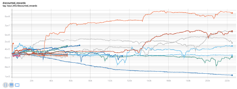
Wow, it looks like our robot is very profitable! Our best robots can even achieve 1000x balance over 200,000 steps, with the rest increasing by at least 30 times the average!

At that moment, I realized there was a glitch in the environment... and after fixing it, this is the new reward chart:

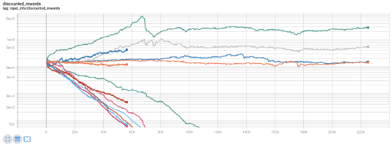
As you can see, some of our robots are doing well and the rest are going bankrupt themselves. However, the best performing robots can only reach 10 times or even 60 times the initial balance. I must admit that all profitable robots are trained and tested without commissions, so it is impractical for our robots to make any real money. But at least we have found a direction!

Let's test our robots in a test environment (using new data they've never seen before) and see how they perform.

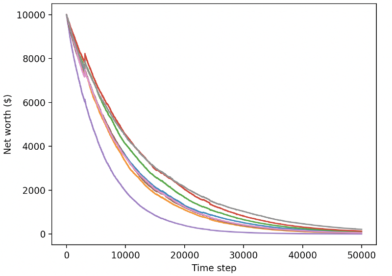
Our highly trained robots will go bankrupt trading new test data.

Obviously, we still have a lot of work to do. By simply switching the model to use stable baseline A2C instead of the current PPO2 robot, we can dramatically improve our performance on this dataset. Finally, according to Sean O'Gorman's suggestion, we can slightly update our reward function so that we add rewards in net worth instead of just achieving high net worth and staying there.

reward = self.net_worth - prev_net_worth

These two changes alone can dramatically improve the performance of the test datasets, and as you'll see below, we're finally able to take advantage of new data that the training sets don't have.

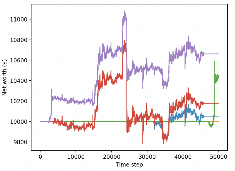
However, we can do better. To improve these results, we need to optimize our hyperparameters and train our robots for longer. It's time to get the GPU working and firing at full power!

By now, this article is a bit long and we still have a lot of details to consider, so we intend to take a break here. In the next article, we will use Bayesian optimization to sort out the best hyperparameters for our problem space and prepare for training/testing on GPUs using CUDA.

Conclusions

In this article, we started using reinforcement learning to create a profitable Bitcoin trading robot from scratch.

1.使用OpenAI的gym从零开始创建比特币交易环境。

2.使用Matplotlib构建该环境的可视化。

3.使用简单的交叉验证对我们的机器人进行训练和测试。

4.略微调整我们的机器人以实现盈利

Although our trading robot is not as profitable as we hoped, we are moving in the right direction. Next time, we will make sure that our robot always beats the market and we will see how our trading robot handles real-time data. Please keep an eye on my next post, and long live Bitcoin!

Related

More