Neural network and digital currency quantitative trading series ((1) LSTM predicts Bitcoin price

1.简单介绍

Deep neural networks have become increasingly popular over the years and have shown powerful capabilities in solving problems that could not be solved in the past in many areas. In time series prediction, the most commonly used neural network price is RNN, because RNN has not only current data input, but also historical data input, of course, when we talk about RNN price prediction, we often talk about a type of RNN: LSTM. This article will build a model of predicting the price of Bitcoin based on pytorch. This tutorial is provided by FMZ inventor digital currency quantification trading platform (((((((((((((((((((((((((((((((((((((((((((((((((((((((((((((((((((((((((((((((((((((((((((((((((((((((((((((((((((((((((((((((((((((((((((((((((((((((((((((((((((((((((((((((((((((((((((((((((((((((((((((((((((((((((((((((((((((((((((((((((www.fmz.comIn the meantime, I'm going to share some of my thoughts on this topic with you.

2.数据和参考

Bitcoin price data is sourced from the inventor of FMZ's quantitative trading platform:https://www.quantinfo.com/Tools/View/4.htmlA related price forecast example:https://yq.aliyun.com/articles/538484A detailed introduction to the RNN model:https://zhuanlan.zhihu.com/p/27485750Understanding the input and output of RNN:https://www.zhihu.com/question/41949741/answer/318771336About pytorch: official documentshttps://pytorch.org/docsYou can search for more information here. In addition, reading this article requires some prior knowledge, such as pandas/reptiles/data processing, but it doesn't matter.

Parameters of the pytorch LSTM model

Parameters for LSTM:

The first time I saw these tightly packed parameters in the document, my reaction was:I'm going to read it slowly and I'll probably understand.

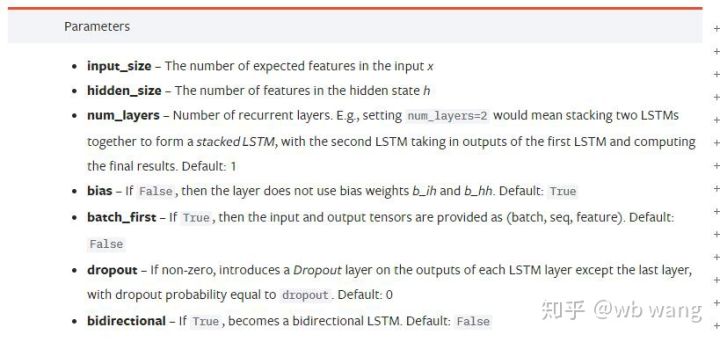
input_size: the characteristic size of the input vector x, if the closing price is predicted at the close, then the input_size = 1; if the closing price is predicted at the close, then the input_size = 4hidden_sizeImplied layer size:num_layersRNN: number of layersbatch_first: This parameter can also be confusing if the first dimension to be entered for True is batch_size, which will be explained in detail below.

Enter the data parameters:

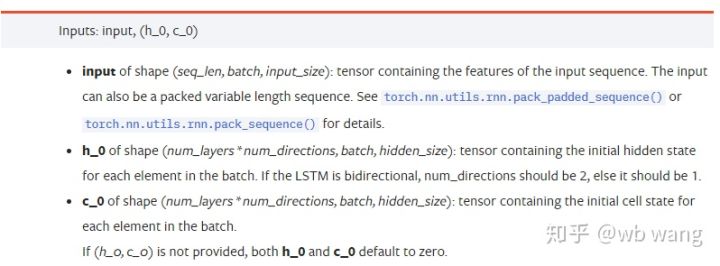
input: The specific input data is a three-dimensional tensor, specifically shaped as follows: ((seq_len, batch, input_size)); wherein, the length of the sequence sequence of sec_len, i.e. LSTM needs to consider how long the historical data is, note that this refers only to the format of the data, not the structure within the LSTM, the same LSTM model can input different sec_len data, all can give the predicted results; batch indicates the size of the batch, representing how many groups of different data; input_size is the previous input_size.h_0: Initial hidden state, shaped as ((num_layers * num_directions, batch, hidden_size), if the bidirectional network number_directions=2c_0: Initial cell state, same shape, can be unspecified.

The output parameters are:

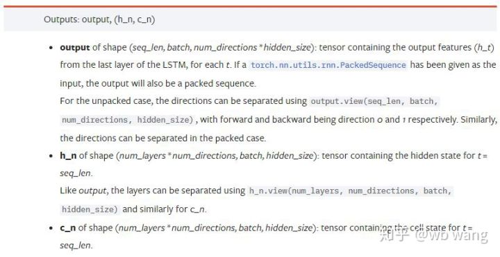
output: output shapes (seq_len, batch, num_directions * hidden_size), note related to model parameter batch_firsth_n: t = seq_len at the moment of h, with the same shape as h_0c_n: t = state c at the moment seq_len, with the same shape as c_0

4.LSTM输入输出的简单例子

First, import the packages you need.

import pandas as pd
import numpy as np
import torch
import torch.nn as nn
import matplotlib.pyplot as plt

Defining the LSTM model

LSTM = nn.LSTM(input_size=5, hidden_size=10, num_layers=2, batch_first=True)

Data ready to be entered

x = torch.randn(3,4,5)
# x的值为:
tensor([[[ 0.4657,  1.4398, -0.3479,  0.2685,  1.6903],
         [ 1.0738,  0.6283, -1.3682, -0.1002, -1.7200],
         [ 0.2836,  0.3013, -0.3373, -0.3271,  0.0375],
         [-0.8852,  1.8098, -1.7099, -0.5992, -0.1143]],

        [[ 0.6970,  0.6124, -0.1679,  0.8537, -0.1116],
         [ 0.1997, -0.1041, -0.4871,  0.8724,  1.2750],
         [ 1.9647, -0.3489,  0.7340,  1.3713,  0.3762],
         [ 0.4603, -1.6203, -0.6294, -0.1459, -0.0317]],

        [[-0.5309,  0.1540, -0.4613, -0.6425, -0.1957],
         [-1.9796, -0.1186, -0.2930, -0.2619, -0.4039],
         [-0.4453,  0.1987, -1.0775,  1.3212,  1.3577],
         [-0.5488,  0.6669, -0.2151,  0.9337, -1.1805]]])

And the shape of x is ((3, 4, 5) as we defined before.batch_first=TrueThe size of the batch_size at this time is 3, sqe_len is 4, input_size is 5; x[0] represents the first batch.

If batch_first is not defined, defaulting to False, then the representation of the data at this time is completely different, batch size is 4, sqe_len is 3, input_size is 5; at this time x[0] represents all batch data at t=0, respectively. Individuals feel this setting is not intuitive, so parameters are added.batch_first=True.

It's also easy to convert data between the two:x.permute(1,0,2)

Input and output

The shape of the input and output of LSTMs can be easily confusing, and the following diagram can help you understand: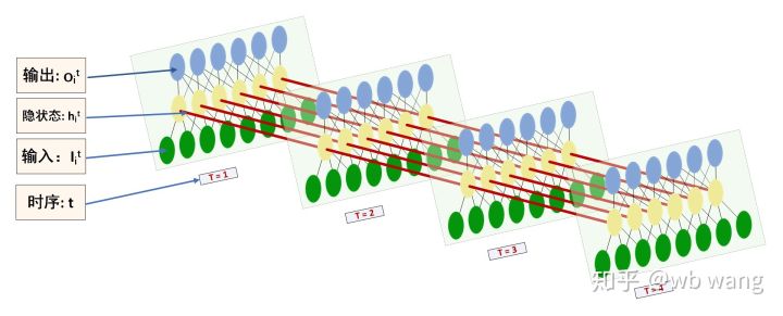
The source:https://www.zhihu.com/question/41949741/answer/318771336

x = torch.randn(3,4,5)
h0 = torch.randn(2, 3, 10)
c0 = torch.randn(2, 3, 10)
output, (hn, cn) = LSTM(x, (h0, c0))
print(output.size()) #在这里思考一下,如果batch_first=False输出的大小会是多少?
print(hn.size())
print(cn.size())
#结果
torch.Size([3, 4, 10])
torch.Size([2, 3, 10])
torch.Size([2, 3, 10])

The results of the observed output are consistent with the explanation of the previous parameters. Note that the second value ofhn.size (()) is 3, and the batch_size size is consistent, indicating that no intermediate state is stored inhn, only the last step. Since our LSTM network has two layers, in fact the output of the last layer is the value of the output, the output is of the form [3, 4, 10], which stores the result of t = 0, 1, 2, 3 at all times, so:

hn[-1][0] == output[0][-1] #第一个batch在hn最后一层的输出等于第一个batch在t=3时output的结果
hn[-1][1] == output[1][-1]
hn[-1][2] == output[2][-1]

5.准备比特币行情数据

It is important to understand the input and output of LSTM, otherwise it is very easy to get some code from the Internet, because due to LSTM's strong ability on the time series, even if the model is wrong, it can end up with good results.

Access to data

The data used is market data for the BTC_USD trading pair on the Bitfinex exchange.

import requests
import json

resp = requests.get('https://www.quantinfo.com/API/m/chart/history?symbol=BTC_USD_BITFINEX&resolution=60&from=1525622626&to=1562658565')
data = resp.json()
df = pd.DataFrame(data,columns = ['t','o','h','l','c','v'])
print(df.head(5))

The data format is as follows: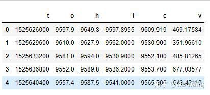

Pre-processing of data

df.index = df['t'] # index设为时间戳
df = (df-df.mean())/df.std() # 数据的标准化,否则模型的Loss会非常大,不利于收敛
df['n'] = df['c'].shift(-1) # n为下一个周期的收盘价,是我们预测的目标
df = df.dropna()
df = df.astype(np.float32) # 改变下数据格式适应pytorch

The method of standardizing data is very rough and there are some problems, just a demonstration, which can be used to standardize data such as yield rates.

Preparing training data

seq_len = 10 # 输入10个周期的数据
train_size = 800 # 训练集batch_size
def create_dataset(data, seq_len):
    dataX, dataY=[], []
    for i in range(0,len(data)-seq_len, seq_len):
        dataX.append(data[['o','h','l','c','v']][i:i+seq_len].values)
        dataY.append(data['n'][i:i+seq_len].values)
    return np.array(dataX), np.array(dataY)
data_X, data_Y = create_dataset(df, seq_len)
train_x = torch.from_numpy(data_X[:train_size].reshape(-1,seq_len,5)) #变化形状,-1代表的值会自动计算
train_y = torch.from_numpy(data_Y[:train_size].reshape(-1,seq_len,1))

The shape of the final train_x and train_y are: torch.Size (([800, 10, 5]), torch.Size (([800, 10, 1]) ; since our model predicts the closing price of the next cycle based on data from 10 cycles, theoretically 800 batches would work as long as there are 800 predicted closing prices. But there are 10 data in each batch, and in fact the intermediate results of each batch are reserved, not just the last one. When calculating the final loss, all 10 predictions can be taken into account and the actual value in train_y is compared.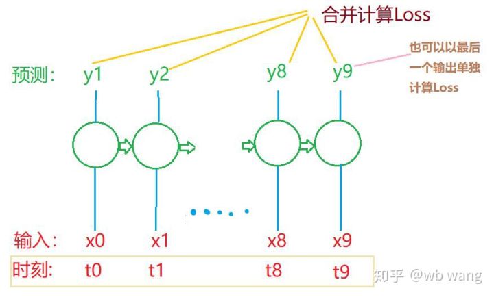

Note that when preparing the training data, the movement of the window is jumpy, the data that has already been used is no longer used, and of course the window can also be moved individually, which results in a large training assembly.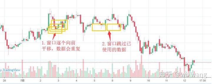

6.构造LSTM模型

The final model was constructed as follows, containing a two-layer LSTM, a Linear layer.

class LSTM(nn.Module):
    def __init__(self, input_size, hidden_size, output_size=1, num_layers=2):
        super(LSTM, self).__init__()
        self.rnn = nn.LSTM(input_size,hidden_size,num_layers,batch_first=True)
        self.reg = nn.Linear(hidden_size,output_size) # 线性层,把LSTM的结果输出成一个值

    def forward(self, x):
        x, _ = self.rnn(x) # 如果不理解前向传播中数据维度的变化,可单独调试
        x = self.reg(x)
        return x
        
net = LSTM(5, 10) # input_size为5,代表了高开低收和交易量. 隐含层为10.

7.开始训练模型

The code is as follows:

criterion = nn.MSELoss() # 使用了简单的均方差损失函数
optimizer = torch.optim.Adam(net.parameters(),lr=0.01) # 优化函数,lr可调
for epoch in range(600): # 由于速度很快,这里的epoch多一些
    out = net(train_x) # 由于数据量很小, 直接拿全量数据计算
    loss = criterion(out, train_y)
    optimizer.zero_grad()
    loss.backward() # 反向传播损失
    optimizer.step() # 更新参数
    print('Epoch: {:<3}, Loss:{:.6f}'.format(epoch+1, loss.item()))

The results of the training are as follows: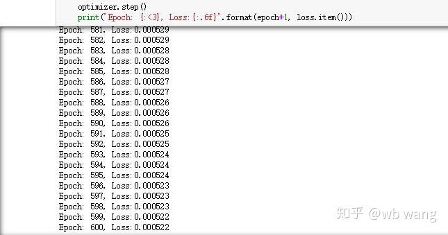

8.模型评价

The model predicts:

p = net(torch.from_numpy(data_X))[:,-1,0] # 这里只取最后一个预测值作为比较
plt.figure(figsize=(12,8))
plt.plot(p.data.numpy(), label= 'predict')
plt.plot(data_Y[:,-1], label = 'real')
plt.legend()
plt.show()

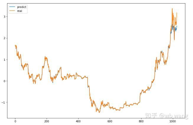
As can be seen from the graph, the correspondence between the training data ((before 800) is very high, but the price of Bitcoin has risen significantly in recent years, and the model has not seen these data, so the prediction is not correct. While the price forecast is not always accurate, what about the accuracy of the fall?

r = data_Y[:,-1][800:1000]
y = p.data.numpy()[800:1000]
r_change = np.array([1 if i > 0 else 0 for i in r[1:200] - r[:199]])
y_change = np.array([1 if i > 0 else 0 for i in y[1:200] - r[:199]])
print((r_change == y_change).sum()/float(len(r_change)))

The result is 81.4% accuracy, which is better than I expected.

This model, of course, has no practical value, but it is simple and easy to understand, which is just an introduction to the future of neural networking.