Expected gains from high-frequency trading

Expected gains from high-frequency trading

Summary

The definition of α in high-frequency trading is more complex than in low-frequency trading, as not all strategies are predictive based on price, but require more conditions and an understanding of the interactions between them. In this article, we develop an α attribution model of high-frequency trading by explaining the components of high-frequency trading and the trading strategies used to implement the high-frequency strategy. The results show that high-frequency traders need to be fast to generate positive expected returns, and why they are better at providing liquidity.

In high-frequency trading (HFT), the expected return is the key to profitability. Usually, this expectation is called alpha (α) {\displaystyle alpha (α) } {\displaystyle (α) } {\displaystyle (α) } {\displaystyle (α) } {\displaystyle (α) } } {\displaystyle (α) } {\displaystyle (α) } {\displaystyle (α) } {\displaystyle (α) } {\displaystyle (α) } {\displaystyle (α) } {\displaystyle (α) }} {\displaystyle (α) } {\displaystyle (α) } {\displaystyle (α) }}} {\displaystyle (α) } {\displaystyle (α) } {\displaystyle (α) } } {\displaystyle (α) } } {\displaystyle (α) } } In low-frequency trading, alpha is equal to volatility times the information coefficient (IC) {\displaystyle (z) } {\displaystyle (z) } {\displaystyle (z) } {\displaystyle (IC) } {\displaystyle (z) } } {\displaystyle (z) } {\displaystyle (z) } {\displaystyle (z) } {\displaystyle (z) } } {\displaystyle (Grinold[1994]) } {\displaystyle (Grin

In this paper, we developed an α-attribute model for high-frequency trading. We achieve this by explaining the components of α, as well as the trading strategies used to implement HFT strategies. These components include:

1. The Opportunity
2. Acquisition
3. The Effective Difference
4. This is a very good thing.

In addition, we provide an implementation example using high-frequency stock data samples.

α in HFT

The HFT industry often defines α with absolute returns of 1; the average absolute returns generated by retracement or simulation transactions (based on each transaction or per unit of time) should properly be called retracement test α or simulation α. We will of course use retracement and/or simulation α as a reason to believe in the future α (i.e., once the strategy starts to run); breaking these α down into its components allows for improvements in the trading strategy, or, as is usually the case, an after-the-fact analysis of why the strategy deviates from the expected performance.

Perhaps if we start from the perspective of high-frequency strategies, as with low-frequency strategies, it is mainly to profit by eliminating inefficiencies in the market. In doing so, it is necessary to be aware of the same basic ideas that affect all investment strategies: how many opportunities can be seized; how much can be obtained; what is the cost of obtaining it?

Opportunities

The starting point for any discussion of α is the available price change or opportunity (O) ─ price change in a given holding period represents the available profit (O) ─ a common way of measuring this change is the standard deviation of the buy/sell intermediate price change (BPD) ─ standard deviation is of course an appropriate measure for portfolio strategies that require continuous market exposure, but for opportunistic HFT strategies (entering positions only under certain conditions) different opportunity measurement criteria may be appropriate (e.g., in futures trading, a 90-digit change, or even a fixed number of cents or hands); however, in the absence of other measurement criteria, we recommend using standard deviation as an opportunity.

Acquisition (C)

We will define gain (C) as the percentage of opportunity that can be gained by any strategy other than the predictive signal; gain is the IC×z score (see Grinold[1994]) in the case of portfolio strategies, which is often used to measure the correlation between predictive returns and actual earnings achieved. Because IC is based on price prediction, any negative of IC is bad. However, in HFT, a negative of C is likely to be acceptable because other measures may be more appropriate than correlation.

Effective difference (SE)

In low-frequency trading, the bid/ask spread is often overlooked as a component of the α, because the opportunity sought is much larger. However, in HFT, the holding period is short and the bid/ask spread has a big impact on the α. The bid/ask spread is simply the difference between the bid/ask price (the price received by the person who needs to sell immediately) and the ask price (the price paid by the person who needs to buy immediately). In the traditional sense, as stated in Stoll (1978), it is considered to be the premium paid to market makers because they assume the risk of reverse selection when trading with knowledge.

交易策略是指交易策略如何使用市价订单和限价订单来进入和退出金融工具的头寸。限价单是一种要求以低于（高于）账面最高买入（卖出）价进行交易的价格。这样的订单向市场的一方（无论是买入方还是卖出方）提供了流动性。限价订单是被动的，在它们与传入的有价卖出（买入）订单相匹配之前，一直留在交易所的限价订单簿中。市价单是指要求立即以最佳买入（卖出）价格立即进行交易的任何请求。此类订单需要流动性，并以市场价格为准。市价单可以是市价订单，也可以是价格超过账面最高出（卖）价4的限价订单.

A combination of take-and-go orders or hang orders defines three trading strategies. The take-take strategy uses two sellable orders to enter and exit the market position. The make-take strategy uses a limit order to enter and exit the market position. The make-make strategy uses one limit order to enter and exit the market position. Different strategies produce different bid/ask costs.

For example, consider a simple market, as shown in Figure 1; the internal market, the highest point on the ledger, is 99 bids and 100 ask prices, with a bid-ask spread of only 1;; (For simplicity's sake, we ignore the numbers at these levels;;) a take-take strategy, where a position is bought at a market price of 100 and then sold immediately at a market price of 99, only to lose one point by producing a bid-ask spread price S.

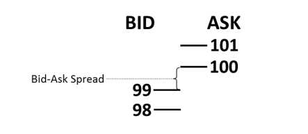
Figure 1: A simplified market with a price difference

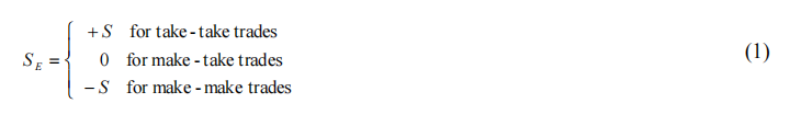
A trade strategy using make-take, whereby a position is bought at 99 points on a limit order and then immediately exited the position and sold at 99 points at the market price, does not generate the cost of the bid/ask spread. Lastly, using make-make trading, whereby a position is entered on a limit order, bought at 99 points and then immediately entered and sold at 100 points on a limit order at some later time, obtains the bid/ask spread S. These simple scenarios result in the effective spread in equation 1).

Effective withdrawal (RE)

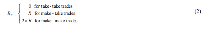
In the stock market, exchanges typically pay a fee to liquid trading firms for providing liquidity by placing a limit order in the limit order book, known as a rebate (R); incentive liquidity providers are considered to have all the profits on the transaction. Having a deeper, more liquid market should attract more, larger institutional liquidity recipients, thus increasing trading volume and exchange fees. When executing or matching a limit order, the trading firm earns R. Therefore, rebate can be an important part of the transaction.

Expected earnings (α)

Given these four components, the α of the HFT strategy can now be fully defined as:

In formula ((3)), α is equal to the net cost of trading minus the opportunity gained. It ignores commissions and collateral, whereas in HFT, commissions and collateral are usually fixed. For example, securities traders are not concerned with commissions, and high-frequency traders who enter the market directly usually pay a fixed fee per share. If these are important variables in a company's decision-making strategies, they can easily be added to formula ((3)).

The importance of strategy

In the formula ((3)), the complexity is that the values of the parts are interdependent. There is a hidden interaction. If we take this into account, the opportunity to obtain is not independent of the effective difference:

1) Capture is the function of entering a position quickly and leaving it as close to the optimal time as possible. 2) The effective spread is a function of the trading strategy employed. The spread can be executed and paid for immediately, or the spread can be earned by waiting for the market to execute a passive limit order.

Therefore, to obtain an effective spread, some of the opportunities already gained must be sacrificed. Or, to obtain more opportunities means to pay the effective spread. The strategy is important because the percentage of gain C decreases with the speed of execution. If we consider the trading strategy implemented in these three ways, we can see the effect of the strategy on α. We assume that the trading strategy has the following characteristics:

• The average holding time is 60 seconds.
• The average bid/ask spread S is 0.08, or 8 cents.
• The odds of a standard deviation of O60 over a 60-second holding period are 0.09, or 9 cents.
• R is 0.001, or one tenth of a penny.

Example 1: Take-Take

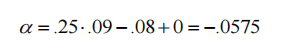
If the strategy uses the take-take strategy, the effective price difference SE is 0.08, and RE is 0; if C is 0.25, then the strategy's α is -0.0575; the result of taking the take-take strategy is to execute and capture all C×O immediately, but it will produce an S-value; therefore, C×O must be greater than S in order to have a profitable strategy.

Example 2: Make-Take

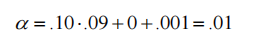
If the strategy uses the make-take strategy, the effective price difference SE is 0, RE is 0.001; if C is reduced to 0.10, then the strategy's α is 0.01. The make-take strategy does not cause a slide, but will cause an unknown delay before the trade is opened. The C value has fallen due to the execution of delays and reverse options. Therefore, traders using the make-take strategy in the strategy should minimize the waiting time in the price list queue.6

Example 3: Make-Make

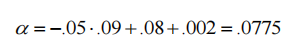
If the strategy uses the make-make strategy, the effective price difference SE is -0.08, RE is 0.002; if C is -0.05, then the α of the strategy is 0.0775; C's value decreases further due to the waiting time of the trading parties and the reverse selection of the parties. In this case, even if C is negative, the difference and rebate will also make the expected value positive. The make-make strategy is compensated by the amount of S and the waiting time of 2×R, so even if C is negative, the strategy still has a positive α.

This situation paints a good picture for a strategy that provides liquidity. It does not take into account that this strategy occasionally produces extreme left-end gains when a reverse option event occurs, especially if the technique is slow. This situation leads to new trading strategies with very short holding periods, with C values kept close to zero, both of which help to reduce the likelihood of reverse options, so α is for S+RE. Example 3 shows why HFT strategies are better at providing low liquidity than low-frequency traders.

Experience 7 and results

To demonstrate the properties of formula (1) and the effect of various strategies on α, we used data from Apple (AAPL) dated January 3, 2012. We tried various examples, but no qualitative change occurred. The dataset contains all the information for each event in the Nasdaq limit price order sheet, including all add, subtract and execute operations. The timing of this information is nanoseconds, so we can accurately time and order all events. Using this data, we use the standard for the change in the price of the bid-offer spread over a period of time to calculate the opportunity.

Using the data just described, the average buy/sell spread S on the day was 0.088704, about 9 cents. The USD standard deviation for different holding periods is shown in Figure 2.

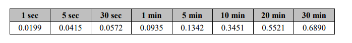
Figure 2: Standard deviation of different holding periods

Using the standard deviation in Figure 2 as a proxy for the odds, we calculate the value of α for C using the formula ((3)), which ranges from −1 to 1。(C=1 is logically equivalent to the case of Kearns et al. in the case of the jack of all trades,[2010]。) We assume R=0。Figures 3, 4, and 5 show three strategies in different holding periods α。 For example, in Figure 3 if the holding period is 1 second, C=-1.00, O=0.0199, S=0.088704, and R=0, then for the take-take tactic, α is −0.109, as shown in the upper left corner. In Figure 3-5, each shadow element represents the value of α as positive in all other elements, or α as negative.

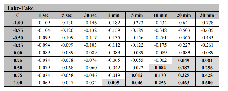
Figure 3: Take-Take strategy provided by Alphas

In Figure 3, we can see that for take-take strategies, α is positive only when the C-value is incredibly high (i.e. 0.75 or 1.00), or when the holding period is quite long, at least by HFT standards. In practice, a high C-value can be used for strategies that chase slightly fleeting opportunities. For strategies that rely on price forecasting, C-value above about 0.25 is difficult to detect, and holding periods of 20 to 30 minutes may be outside the high-frequency definition range.

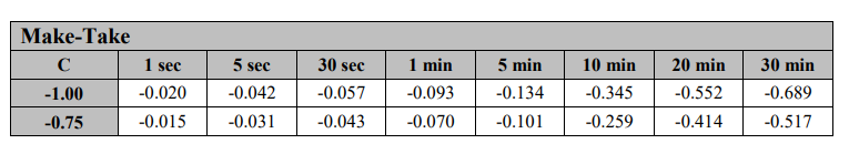
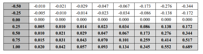
Figure 4: The Make-Take strategy provided by Alpha

In Figure 4, we can see that for the make-take strategy, α is positive under any positive value; this is very clear, because when S = 0, the current gain leads to positive α, and the negative gain leads to negative α. However, the implicit assumption is that the waiting time in the queue is short. Orders usually stay in the queue for a few seconds, or even minutes, which excludes obtaining α in these time frames. Of course, the faster a person's technique, the faster his order is in the queue, and therefore, the waiting time is shorter.

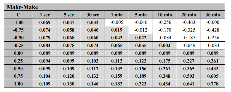
Figure 5: Make-Make strategy provided by Alphas

In Figure 5, we can see that for make-make strategies, α is positive in almost all values of C. Even if C is negative, the value of the price difference can basically overcome any strategy, no matter how fast the technique is. As in the previous example, obtaining positive α associated with the shorter holding period depends on whether the limit order can be executed quickly. This can only occur if the shorter the waiting time, which means that you are always at the front of the queue.

The Effect of Speed

The speed of the technology has a profound effect on the opportunities gained. First, as shown in Figure 6, the correlation between the forecast and the actual price changes decreases over time. This decrease is a function of the forecast length. Figure 6 shows decreases in forecasts of 1 second and 5 seconds in the case of a tenth-second delay. Therefore, any delay in execution will have a negative impact on acquisition.

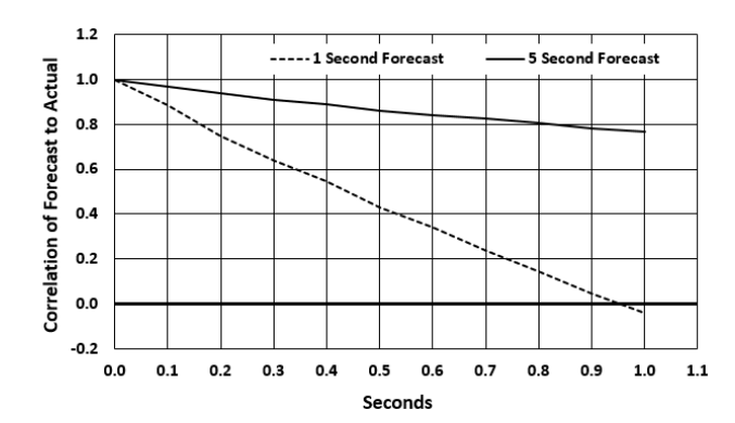
Figure 6: Predicted decline over time

Second, execution delays can affect the calculation of opportunity; speed can be slow and lead to queue lag; trades in the back of the queue tend to be easier to execute compared to informed trades (erroneous direction); reverse selection is more likely and the opportunity to execute will be worse than shown by the simple standard deviation; it is unfortunate for a strategy with negative gain C; it may require a take trade to stop the cumulative loss, producing a worse effective price difference than a make-make strategy; thus, the profitability of the strategy using the make-make strategy in Figure 5 is illusory, except for very fast players.

Conclusions

HFT strategies face a complex expected return formula; however, by breaking down α into its components, trading firms can better understand the variability of profit and loss. Of course, this variability includes not only the variability of the components, but also the correlations that must be considered. These correlations explain the need for speed. Technical speed helps prevent components from forming large negative correlations, causing rapid spiral declines.

References

Grinold, R. C. “Alpha is volatility times IC times score.” Journal of Portfolio Management, 20 (1994), pp. 9-16. Stoll, H. R. “The supply of dealer services in securities markets.” Journal of Finance, 33 (1978), pp. 1133-1151. Kearns, M., A. Kulesza, Y. Nevmyvaka. “Empirical limitations on high frequency trading profitability.” Journal of Trading, 5 (2010), pp. 50-62.

1. Some strategies may also involve residual gains relative to the benchmark. In this case, our approach is easy to apply.
2. The bid-ask spread is the bid-ask spread divided by two. The standard deviation is usually the standard deviation of the logarithmic gain, but we use dollars.
3. For low-frequency strategies, C×O would be exactly the same as what Greenold (1984) said.
4. If the price of the purchase order is equal to or higher than the highest price on the current ledger, it is not placed on the trading order book but is immediately matched with the remaining order at the market sale price.
5. The take-make strategy is rarely (if ever) used in HFT.
6. We assume an advanced first-in-first-out (FIFO) queue with price and time priority.
7. Thanks to Xambala, Inc. for providing this data, and with permission from Nasdaq to use it in our research.
8. A complicated issue we have not yet solved is that reverse options associated with large-disc fluctuations can lead to surrender stop-loss trades, which is another reason why speed of execution is important.

The original address:https://papers.ssrn.com/sol3/papers.cfm?abstract_id=2553582