

I have recently become interested in relative-value and arbitrage strategies. In an earlier example, we traded EWY against Samsung Electronics and SK Hynix. That trade, however, depended on a human being first recognizing the economic relationship.
Can we automate the search itself—screening the market for baskets that may contain a tradable relative-value structure?
This article develops one possible workflow.
1. What Did the EWY Trade Really Cost?
Let us first clarify the earlier example.
EWY is a South Korea ETF, and Samsung Electronics and SK Hynix are among its most important constituents. If EWY becomes expensive relative to those constituents, the trade is to short EWY, go long the constituents, and wait for the relative prices to move back toward their previous relationship.
There is nothing wrong with that idea. But it contains a hidden cost that is rarely measured: how much prior knowledge did you need before you could even identify those three instruments?
You had to know that EWY tracks South Korea. You had to know that Samsung and SK Hynix carry large weights. You had to understand how the memory-chip cycle propagates through the group. You also had to estimate how much the Korean won could contaminate the spread.
None of that information sits directly inside a price matrix. It sits in your head.
That knowledge is an asset accumulated over many years. But precisely because it is a human asset, it is difficult to replicate, scale, or delegate to a machine.
That is the motivation for the entire strategy:
A market may contain hundreds of instruments, tens of thousands of pairs, and millions of three-name combinations. How many can one person examine?
The ceiling of pair trading is not necessarily its return. The ceiling is that a human can only reason carefully about a limited number of relationships at once.
The goal here is to take the step of deciding which instruments belong together away from manual selection and turn it into a process that can be rerun every day.
2. Step One: Arrange Prices as a Matrix
Everything begins with a simple operation: place prices into a table.
- Rows represent time.
- Columns represent instruments.
- Each cell contains a log price.
python
P = np.array([[series[s][t] for s in kept] for t in ts], dtype=float)
L = np.log(P) # T × N log-price matrix
The logarithm is not cosmetic. Relative-value trading is fundamentally concerned with ratios, and logarithms convert ratios into differences.
A move from 10 to 20 and a move from 100 to 200 produce the same log return. Only after this transformation do later linear operations—weighting, projection, and regression—have a consistent interpretation.
This matrix, with T rows and N columns, becomes the object on which the rest of the workflow operates. Its structure determines whether the instruments contain a potentially tradable relative relationship.
3. Ten Semiconductor Instruments May Really Be One
Consider a ten-instrument semiconductor-related basket. A typical candidate set may include AMD, ARM, ASML, INTC, MRVL, NVDA, TSM, QQQ, SPY, and another instrument admitted by the screen.
Visually, the columns often look highly similar: when one rises, most of the others rise; when one falls, most of the others fall.
In linear algebra, this is described as low rank. The matrix may have ten columns, but its effective number of common degrees of freedom may be much smaller.
Singular value decomposition provides a way to separate those directions:
            python

            _, S, Vt = np.linalg.svd(Xc, full_matrices=False)
V  = Vt.T
Vf = V[:, :k]      # estimated common-trend directions
Vn = V[:, k:]      # estimated residual subspace
Choosing k is the first genuinely difficult question.
- If
kis too small, real common movement is treated as noise and directional market exposure remains in the basket. - If
kis too large, noise is promoted to a factor and the system trades a structure that may not exist.
The implementation uses a Marchenko–Pastur upper-edge rule as a practical factor-count heuristic. Under its random-matrix assumptions, eigenvalues above the noise edge are treated as candidate common factors:
            python

            def mp_factor_count(returns):
    T, N = returns.shape
    q = float(N) / float(T)
    upper = (1.0 + math.sqrt(q)) ** 2    # upper edge under the noise model
    ev = np.linalg.eigvalsh(C)
    return int(np.sum(ev > upper))       # count eigenvalues above the edge
This rule automatically responds to sample size through q = N/T. A shorter training window or a larger universe raises the noise edge and makes the filter stricter.
That is directionally sensible: when data are scarce, the model should be less willing to believe that an apparent structure is real.
In one run, the result was k = 1.
In other words, the basket was largely driven by one common movement, with the remaining dimensions representing relative deviations.
The Marchenko–Pastur edge should still be treated as a heuristic rather than a proof. Financial returns are not independent Gaussian noise, and temporal dependence, heavy tails, and volatility clustering can change the empirical eigenvalue spectrum.
4. The Residual Subspace: Several Distinct Relative-Value Directions at Once
This is where the approach begins to differ from ordinary pair trading.
If N = 10 and the estimated number of common trends is k = 1, the remaining N - k = 9 dimensions lie outside the leading common direction.
Under a valid common-trend and cointegration structure, portfolios formed in this residual subspace can suppress much of the shared market movement and leave mainly relative deviations.
If the entire semiconductor group rises 5%, a well-constructed residual portfolio should move much less. If the group falls 8%, the same should be true. What remains is the question of which member moved away from the others.
The earlier EWY trade can be understood as a manually discovered direction in such a space. A human chose weights intended to cancel the broad South Korea exposure and isolate a relative mispricing.
SVD provides multiple candidate directions at once.
However, one distinction matters:
Orthogonal directions are not automatically statistically independent bets.
They are geometrically distinct coordinates in weight space. Their realized residual time series may still be correlated, especially outside a Gaussian model. Covariance whitening and out-of-sample validation are therefore still necessary.
The practical change from pair trading to matrix trading is not merely that more instruments are involved. It is that the strategy monitors a multidimensional residual structure rather than a single spread.
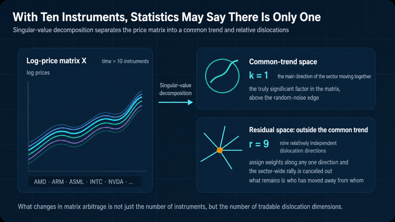
Figure 1 | Matrix arbitrage increases the number of relative-deviation dimensions that can be monitored outside the dominant common trend.
5. Whether the Space Is Usable Depends on Spectral Separation
The output of SVD should not be accepted without a stability check.
SVD orders directions by singular value. The first k directions are assigned to the common-trend space and the remainder to the residual space. The question is whether the boundary between the two is stable.
Suppose the k-th singular value is 100 and the next is 20. The separation is large, so a moderate perturbation is unlikely to change the subspace dramatically.
If the values are 51 and 49, the boundary is fragile. On the next rebuild, a direction may rotate from the residual space into the factor space. A carefully calculated portfolio from yesterday may then represent a substantially different exposure today.
Perturbation results such as the Davis–Kahan and Wedin sin Θ theorems can be summarized schematically as:
            text

            subspace rotation  ≤  perturbation size / absolute spectral separation
The denominator is the separation between the relevant singular-value groups. It is a quantitative stability concept, not a metaphor.
The implementation uses a singular-value ratio as a convenient scale-free proxy:
            python

            gap = float(S[k - 1] / S[k])

if gap < MIN_GAP:                 # default: 1.30
    return None, "insufficient singular-value separation {:.2f}<{:.2f}".format(
        gap, MIN_GAP
    )
Strictly speaking, the perturbation theorem depends on absolute separation relative to perturbation magnitude, not on the ratio alone. The ratio is therefore an engineering filter, not a theorem-level guarantee.
The theoretical screen is followed by an empirical one. The training window is split into two halves, the residual subspace is estimated separately in each half, and the principal angle between the estimates is measured:
            python

            half = eff // 2
angles = []

for seg in (train[:half], train[half:]):
    Sc = seg - seg.mean(axis=0)
    _, _, vt = np.linalg.svd(Sc, full_matrices=False)
    angles.append(principal_angles_deg(Vn, vt.T[:, k:]))

if max(angles) > MAX_ANGLE_DEG:   # default: 20°
    return None, "subspace rotation {:.1f}°>{:.1f}°".format(
        max_angle, MAX_ANGLE_DEG
    )
This test asks a sharp question:
Do the first and second halves of the sample point toward approximately the same relative-value space?
A small angle suggests temporal consistency. A large angle suggests that the apparent structure may be specific to one section of the sample.
Examples rejected by this filter included:
            text

            6   BMNR,COINX,CRCLX,HOODX,MSTRX,ORCLX     subspace rotation 49.6° > 20.0°
6   AMZNX,GOOGLX,IBM,METAX,MSFT,PLTRX      subspace rotation 87.0° > 20.0°
13  AAPLX,AMZNX,BABA,CXMT,FUTUON,GOOGLX    subspace rotation 80.0° > 20.0°
An angle of 87 degrees means the two estimated spaces are almost orthogonal.
This filter often rejects the baskets that look most convincing to the eye. Large technology stocks may be highly correlated, but high correlation is not the same as a stable tradable relationship.
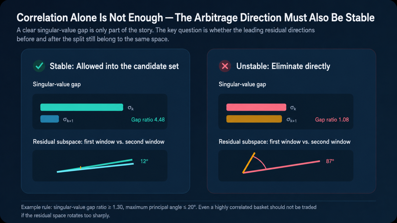
Figure 2 | Singular-value separation tests the boundary between factor and residual spaces; principal angles test whether the estimated residual structure rotates over time.
6. Two Statistics: One Finds Misalignment, the Other Avoids Catching a Falling Knife
Once a basket is admitted, it enters real-time monitoring.
Two statistics are used, and they serve different purposes.
Q-score: How Deep Is the Structural Misalignment?
Project the current log-price vector into the residual subspace and measure its Mahalanobis distance using the residual covariance estimated in training:
            python

            rvec = xc @ Vn
q_raw = float(rvec @ np.array(model["resid_inv"]) @ rvec)
Why use Mahalanobis distance rather than Euclidean distance?
Because residual directions naturally have different volatility scales. One may be highly active while another remains close to zero most of the time. A single absolute threshold would mainly monitor the largest-variance directions and largely ignore the rest.
Mahalanobis distance normalizes the directions by their covariance and places them on a common scale.
If the residual vector is approximately multivariate Gaussian and the covariance matrix is known—or estimated accurately from a much larger sample—the squared Mahalanobis distance is approximately distributed as χ²(r).
This gives distribution-based reference levels:
            python

            "q_entry": float(sps.chi2.ppf(0.995, r)),   # 99.5th percentile: alert
"q_exit":  float(sps.chi2.ppf(0.80,  r)),   # 80th percentile: exit
This is useful because every parameter that can be grounded in a distribution leaves less room for manual optimization.
The qualification matters: cointegration by itself does not imply Gaussian residuals, and using an estimated covariance matrix, autocorrelated observations, heavy tails, or seasonal rescaling makes the exact χ² calibration only approximate. In production, empirical quantiles and forward false-alarm rates should be compared with the theoretical thresholds.
F-shock: Is the Entire Factor Space Being Repriced?
The purpose of this statistic is to prevent the system from taking the right action at the wrong time.
Suppose the Q-score triggers and the system prepares to trade mean reversion. But the Federal Reserve has just released an unexpected statement and the entire semiconductor sector is being repriced.
The prices may not return, because the new level may be economically justified.
The strategy therefore monitors the speed of movement in the common factor itself:
            python

            f = xc @ Vf                          # factor score
d = f - np.array(prev["f"])          # first difference
fshock = float(d @ np.array(model["f_inv"]) @ d)
An entry requires both conditions:
            python

            "alarm":   q > model["q_entry"],      # residual structure is displaced
"blocked": fshock > model["f_limit"], # factor is moving violently: do not enter
The two statistics describe two sides of the same question:
- High Q, low F: the systematic environment is relatively calm, but the relative positions are displaced. This is the intended setup.
- High Q, high F: the systematic environment itself is changing. This is more likely repricing than temporary misalignment.
Classical multivariate statistical process control often assumes stationary variables. Log prices are generally modeled as integrated processes, so the classical formulation cannot simply be copied.
Here, Q is constructed from residual directions that have passed stationarity screening, while F is constructed from first differences of factor scores. Both statistics are moved onto approximately stationary inputs before distance thresholds are applied.
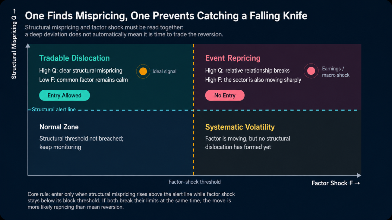
Figure 3 | The preferred region has a large structural displacement but a calm common factor. A simultaneous factor shock is more consistent with event-driven repricing.
7. Attribution: A Residual Belongs to the Basket, Not to One Instrument
A Q-score alert only says that the basket is displaced. It does not identify which instrument caused the displacement.
The residual is created by projection, so it is a property of the portfolio as a whole.
The implementation uses leave-one-out regression for attribution:
            python

            for i in range(N):
    others = [j for j in range(N) if j != i]

    A = np.column_stack([np.ones(eff), train[:, others]])
    b, _, _, _ = np.linalg.lstsq(A, train[:, i], rcond=None)

    res = train[:, i] - A @ b

    loo.append({
        "i": i,
        "others": others,
        "beta": b.tolist(),
        "sd": float(res.std(ddof=1))
    })
The idea is to reconstruct instrument i using the other N - 1 instruments.
- If reconstruction is accurate, instrument
ihas little idiosyncratic displacement. - If its reconstruction residual becomes unusually large, the displacement is attributed to
i.
At run time, each instrument receives a z-score:
            python

            pred = b[0] + float(b[1:] @ x[rec["others"]])
z = (x[rec["i"]] - pred) / rec["sd"]
One live output looked like this:
            text

            ARM:-5.604   NVDAX:-3.099   INTC:2.548   ASML:1.564
ARM was 5.6 standard deviations below the price implied by the other instruments.
The proposed position was therefore:
- long ARM;
- hedge with the remaining legs using the regression coefficients.
            python

            sgn = 1.0 if top["z"] > 0 else -1.0

w = {top["symbol"]: -sgn}

for pos_j, j in enumerate(rec["others"]):
    w[model["members"][j]] = sgn * float(b[1 + pos_j])
The OLS normal equations guarantee that the in-sample regression residual is orthogonal to the regressor columns. That is useful, but it should not be overstated.
It does not by itself guarantee that the live portfolio is neutral to every latent market factor out of sample. A stronger implementation should verify the final weights against the estimated factor loadings or explicitly project the executable portfolio back into the residual subspace.
The leave-one-out residual should also receive its own stationarity check. A basket-level stationary residual space does not automatically imply that every leave-one-out regression residual is stationary.
This is the automated analogue of the EWY triangle—except that it may contain many legs and is rebuilt repeatedly from data.
8. Three Traps: Perfect In Sample, Persistent Losses Out of Sample
The previous sections describe the method. The following traps are more important because each can produce an attractive backtest and a slow live loss.
Trap 1: Path Dependence in Leveraged ETFs
SOXL targets three times the daily return of a semiconductor index. TQQQ targets three times the daily return of the Nasdaq-100.
Their short-horizon correlation with the underlying market can approach 0.99, which makes them appear to be ideal relative-value partners.
But daily rebalancing means:
            text

            ln(3× leveraged ETF)  ≠  3 × ln(underlying)
The difference is path dependent and is influenced by volatility, return autocorrelation, financing costs, fees, and the daily reset mechanism.
In volatile or mean-reverting markets, this often appears as volatility drag. In strongly trending markets, a leveraged ETF may instead outperform a simple long-horizon multiple.
The key point is not that the drift is always deterministically negative. The key point is that high correlation does not imply a stable cointegrating relationship.
One practical screen marks a near-duplicate with much higher volatility as a potential leveraged version:
            python

            if abs(C[i, j]) >= DEDUP_RHO:                    # ρ > 0.97
    hi, lo = (i, j) if vol[i] > vol[j] else (j, i)

    if vol[hi] / vol[lo] >= DEDUP_VOL_RATIO:     # volatility ratio > 1.40
        drop_idx.add(hi)

# Drop SNXX, keep SNDK:
# correlation 0.9813, volatility ratio 2.15×
This only catches pairwise near-duplicates.
SOXL may not reach a correlation of 0.97 with any single constituent, so a second basket-level filter is used:
            python

            med_vol = float(np.median(vols))
out = [
    i for i in range(len(kept))
    if vols[i] > VOL_OUTLIER_MULT * med_vol
]
One log entry showed:
            text

            6  AMD,ARM,INTC,MRVL,SOXL,TSM
   basket too small after removing abnormal-volatility member ['SOXL']
The entire basket was rejected.
That is a reasonable trade-off. The expected damage from a structurally contaminated basket can be larger than the opportunity cost of losing one candidate.
Trap 2: Earnings Gaps Look Exactly Like “Misalignment”
U.S. companies often release earnings after the cash market closes, while these perpetual contracts trade around the clock.
At that moment, the rest of a sector may remain nearly unchanged while one instrument jumps 8%.
To the Q-score and leave-one-out attribution, this can look identical to a textbook relative-value opportunity:
- basket residual surges;
- one instrument's z-score exceeds 6;
- the remaining legs barely move.
But the move may represent permanent repricing. The price does not need to return.
The distinction is not necessarily the size of the move, but its speed. A liquidity imbalance may widen progressively, whereas an event-driven repricing may occur in one step.
            python

            if q - prev["q"] > model["q_entry"] * JUMP_MULT:
    # one-cycle jump exceeds 60% of the alert threshold
    jump_until = now + JUMP_COOL_S    # four-hour cooldown
This filter is imperfect. It will reject some genuine fast dislocations.
But the cost of missing one opportunity is not comparable to the cost of repeatedly fading a permanent earnings repricing. Under that asymmetry, a conservative filter is rational.
Trap 3: Intraday Seasonality Requires More Than One Scale
The perpetual contracts trade 24 hours a day, but the underlying U.S. equities have a defined cash session.
Residual volatility during the U.S. trading session can differ by an order of magnitude from volatility during quiet Asian hours.
If one threshold is estimated from the combined sample:
- it may be too loose during the active session and miss genuine dislocations;
- it may be too tight overnight and create a large number of false alerts.
Simply discarding off-hours data is tempting, but it removes some of the most informative observations. Earnings releases often occur outside the cash session, producing the pure pattern of “one leg jumps while the rest remain still.”
The implementation gives each intraday slot its own scale:
            python

            Q_train = np.einsum("ij,jk,ik->i", Rn, resid_inv, Rn)
slots = ((ts[-eff:] // 3600000) % VOL_SLOTS).astype(int)

for h in range(VOL_SLOTS):
    sel = Q_train[slots == h]

    if len(sel) >= MIN_SLOT_BARS:
        slot_scale[str(h)] = float(np.median(sel)) / q_med_all
The effect appears directly in the monitoring panel:
            text

            Q (seasonally normalized)  10.17
Q (raw)                    14.78
slot factor                 1.453
The raw score was 14.78, but baseline volatility for that time slot was already about 45% higher. After normalization, the score fell to 10.17 and remained below the 18.55 alert line.
Without this adjustment, the same false signal could recur every day.
This median rescaling improves comparability, but it does not preserve an exact chi-square distribution. The final threshold should therefore be validated against empirical false-alarm frequencies.
9. In-Sample Mean Reversion Can Contain Almost No Information
This point deserves to be stated directly:
A beautiful in-sample mean-reversion chart is not evidence that the relationship will mean-revert in the future.
When a residual or z-score is centered and standardized using the same sample, its in-sample mean is forced to zero by construction. That is an algebraic property, not a discovered trading edge.
Even unrelated integrated series can produce attractive fitted residual charts over a selected window.
The only informative test is:
Freeze the parameters estimated from the training window, then observe whether future dislocations actually return.
For that reason, the system places forward validation statistics at the top of the dashboard:
            python

            def validation_stats(store):
    done = [
        a for a in store["alerts"]
        if a.get("resolved") is not None
    ]
    ok = [a for a in done if a["resolved"]]

    return {
        "rate": len(ok) / len(done),  # did Q actually return after the alert?
        "median_min": times[len(times) // 2],
        "excursion": np.mean([
            a["peak_q"] / a["q0"] for a in done
        ]),
    }
The current implementation calls the final field mae, but it computes the mean peak-Q multiple across completed alerts, not the maximum adverse excursion. The label should be changed or the calculation should be changed.
The three statistics answer different questions:
| Metric | What It Measures | What Failure Suggests |
|---|---|---|
| Reversion rate | Fraction of alerts for which Q returns below the exit threshold | If persistently below 50%, the cointegration premise is not supported |
| Median reversion time | How long capital remains tied up | If too long, funding and opportunity cost can consume the spread |
| Peak adverse excursion multiple | How far Q moves against the position before resolution | Determines leverage limits, stop design, and whether the strategy can survive until convergence |
The last metric is easy to overlook.
A strategy may show an 80% reversion rate but still experience excursions of three times the entry displacement. With excessive leverage, it can fail before convergence even when the long-run direction is correct.
Being right and surviving are separate problems.
No singular-value gap, ADF statistic, or attractive chart can override the forward table. Those are admission filters, not conclusions.
Because the system screens many baskets and many residual directions, multiple-testing and selection bias also matter. Forward validation must use genuinely future observations, and the reported reversion rate should be accompanied by sample size and uncertainty intervals rather than treated as certain after only a small number of alerts.
10. The Last Mile: A Correct Signal Can Produce the Wrong Orders
One non-mathematical detail can destroy the entire construction.
Contracts trade in integer quantities.
Suppose the target for one leg is 3.7 contracts. Applying floor produces 3 contracts, an error of about 19%. Repeat that across ten legs and the executable portfolio may no longer resemble the intended neutral portfolio.
The consequence is worse than simply earning slightly less.
Once the hedge ratios are distorted, directional market exposure remains. The strategy may appear to be betting that ARM will converge toward the basket while actually carrying a large semiconductor-sector bet.
Before entry, the implementation measures the cosine similarity between target and executable signed notionals:
            python

            tgt = np.array([w.get(sy, 0.0) for sy in w])

act = np.array([
    legs[sy]["notional"] * (1 if long else -1)
    ...
])

fidelity = float(
    tgt @ act / (norm(tgt) * norm(act))
)

if fidelity < MIN_HEDGE_FID:      # default: 0.97
    return                        # cannot match the hedge: do not enter
This constraint can be inverted to estimate the minimum gross exposure required for the basket to be represented with sufficient accuracy:
            python

            needs.append(float(
    np.max(
        FID_TARGET_CT * gran[nz] * aw.sum() / aw[nz]
    )
))

min_gross = float(np.median(needs))
The dashboard can then show:
            text

            BB136E8   minimum gross exposure $11,938   currently tradable ✅
B90094A   minimum gross exposure  $4,597   currently tradable ✅
If the account is too small, the basket should not be traded.
Forcing the trade does not create “a smaller arbitrage.” It creates a directional position dominated by rounding error.
Funding is another frequently omitted cost.
Carry does not automatically cancel across long and short legs because the contracts may have different funding rates. TradFi perpetuals cannot necessarily be arbitraged directly against the underlying shares, so their basis may contain persistent structural differences.
Funding is therefore a deterministic component of realized spread P&L and must be booked explicitly:
            python

            for sym, leg in pos["legs"].items():
    rate = (
        mk["fundingRate"]
        * dt
        / mk["fundingInterval"]
    )

    acc += (
        notional * rate
        if leg["side"] == "long"
        else -notional * rate
    )

pos["funding_paid"] += acc
11. The Complete Pipeline
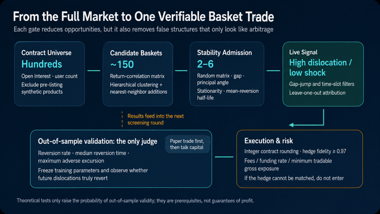
Figure 4 | Screening, validation, monitoring, execution, and forward statistics form a closed loop. Every earlier filter is ultimately judged by out-of-sample results.
            text

            Hundreds of contracts across the market
      ↓  Liquidity gate: open interest and long/short user count
      ↓  Exclude pre-IPO synthetic products
         (no external price anchor, so convergence has no firm basis)

Approximately 120 candidate instruments
      ↓  Hierarchical clustering
         distance = √(2(1−ρ))
         no manually supplied industry labels

Approximately 150 candidate baskets
      ↓  Remove potential leveraged duplicates
      ↓  Estimate factor count k with the MP rule
      ↓  Singular-value ratio ≥ 1.30
      ↓  First-half/second-half principal angle ≤ 20°
      ↓  ADF screening + OU half-life

Approximately 2–6 admitted baskets
      ↓  Real-time Q-score / F-shock monitoring
      ↓  Event-jump filter and intraday seasonal normalization
      ↓  Leave-one-out attribution
      ↓  Integer-contract rounding + hedge-fidelity check

Order construction
      ↓
Forward validation statistics  ← final judge
A sample live output:
            text

            ID       N   k factors   r residual dirs   σ ratio   subspace angle
BB136E8  10  1           6                 4.476     11.96°

best ADF t   half-life   stability score
-5.704       17.8 bars   0.807

AMD, ARM, ASML, INTC, MRVL, NVDA, QQQ, SPY, TSM, ...
The row means:
- the ten instruments were modeled as being driven largely by one common factor;
- six retained residual directions passed the implementation's stationarity screen;
- the singular-value ratio was about 4.5;
- the first-half/second-half residual spaces differed by about 12 degrees;
- the estimated displacement half-life was about 18 bars, or 4.5 hours on 15-minute data.
This is the machine-generated analogue of the EWY triangle: a multi-leg relative-value basket with several residual directions, discovered without manually specifying the economic relationship in advance.
Human choices still remain in universe construction, thresholds, statistical assumptions, execution constraints, and risk limits. The machine automates the search; it does not remove model risk.
12. Four Things That Must Be Stated Clearly
First: There Is No Forced Convergence Mechanism
True arbitrage often has a physical or contractual convergence channel:
- an ETF can be created or redeemed;
- a futures contract expires or settles;
- a convertible claim has enforceable cash flows.
These TradFi perpetual contracts cannot necessarily be exchanged for the underlying U.S. shares.
Their relative prices are constrained mainly by funding rates, market-maker inventory, and quoting conventions. That mechanism is much weaker than physical arbitrage.
This is therefore statistical arbitrage. Convergence is probabilistic, not guaranteed.
Second: Sample Length Is the Largest Weakness
Many of the contracts have short histories and may not have passed through a full earnings cycle.
The current sample cannot establish whether the estimated relationships remain stable across earnings seasons, index rebalances, corporate actions, or changing liquidity regimes.
Forward statistics must continue to accumulate. A few days of paper results are not enough.
Third: Every Theorem and Filter Only Raises the Probability of Forward Validity
The singular-value separation, principal-angle screen, ADF test, OU half-life, and Marchenko–Pastur rule all serve one purpose: improve the chance that the structure survives out of sample.
None provides a guarantee.
They are necessary engineering filters, not sufficient evidence of profitability.
Fourth: Large-Scale Screening Creates Multiple-Testing Risk
The process evaluates many clusters, baskets, directions, thresholds, and attribution candidates.
Even if every individual test uses a 5% significance level, the best-looking survivors can appear significant purely because so many alternatives were tried.
The forward period must remain untouched, rolling evaluation must avoid leakage, and performance claims should include the number of candidates searched and the uncertainty around the observed reversion rate.
The system ultimately reduces to one table:
            text

            🔬 Forward Validation

alerts   completed   reversion rate   median reversion time
1        0           —                —

peak adverse excursion   conclusion
—                        insufficient sample; keep collecting
An operating rule might be:
- if the reversion rate remains above 60% with a sufficiently large sample and acceptable adverse excursion, the premise is worth further risk-budget discussion;
- if it remains below 50%, stop the strategy rather than continuously retuning parameters.
The thresholds themselves are not universal truths. They should be interpreted together with sample size, confidence intervals, transaction costs, and drawdown.
Using parameter changes to manufacture a better historical reversion rate is the definition of overfitting.
Strategy Source
TradFi Matrix Statistical Arbitrage
The strategy is configured for Gate.io by default. Other exchanges may require symbol, metadata, fee, funding, and contract-quantity adaptations.
The default mode is paper, so it does not place real orders.
Accumulate enough out-of-sample evidence before discussing live capital.
Technical Review Notes Before Live Use
The published source should be corrected or strengthened in several places before live deployment:
- Recompute half-life only from the residual directions retained after ADF screening.
- Calculate the ADF pass ratio before overwriting
r; otherwisepass_adf / rbecomes 1 whenever any directions are retained. - Rename the current
maefield or calculate a true maximum adverse excursion; the code currently averagespeak_q / q0. - Test each leave-one-out trading residual for stationarity and verify executable factor exposure; OLS residual orthogonality alone does not ensure live factor neutrality.
- Treat chi-square thresholds as approximate and compare them with empirical forward false-alarm rates after covariance estimation and seasonal normalization.
- Correct the universe-size/member-list inconsistency in the example output.
- Apply multiple-testing controls or nested forward validation when selecting among many baskets and residual directions.
This article is for quantitative research and software-design discussion only. It is not investment advice.
- 1