
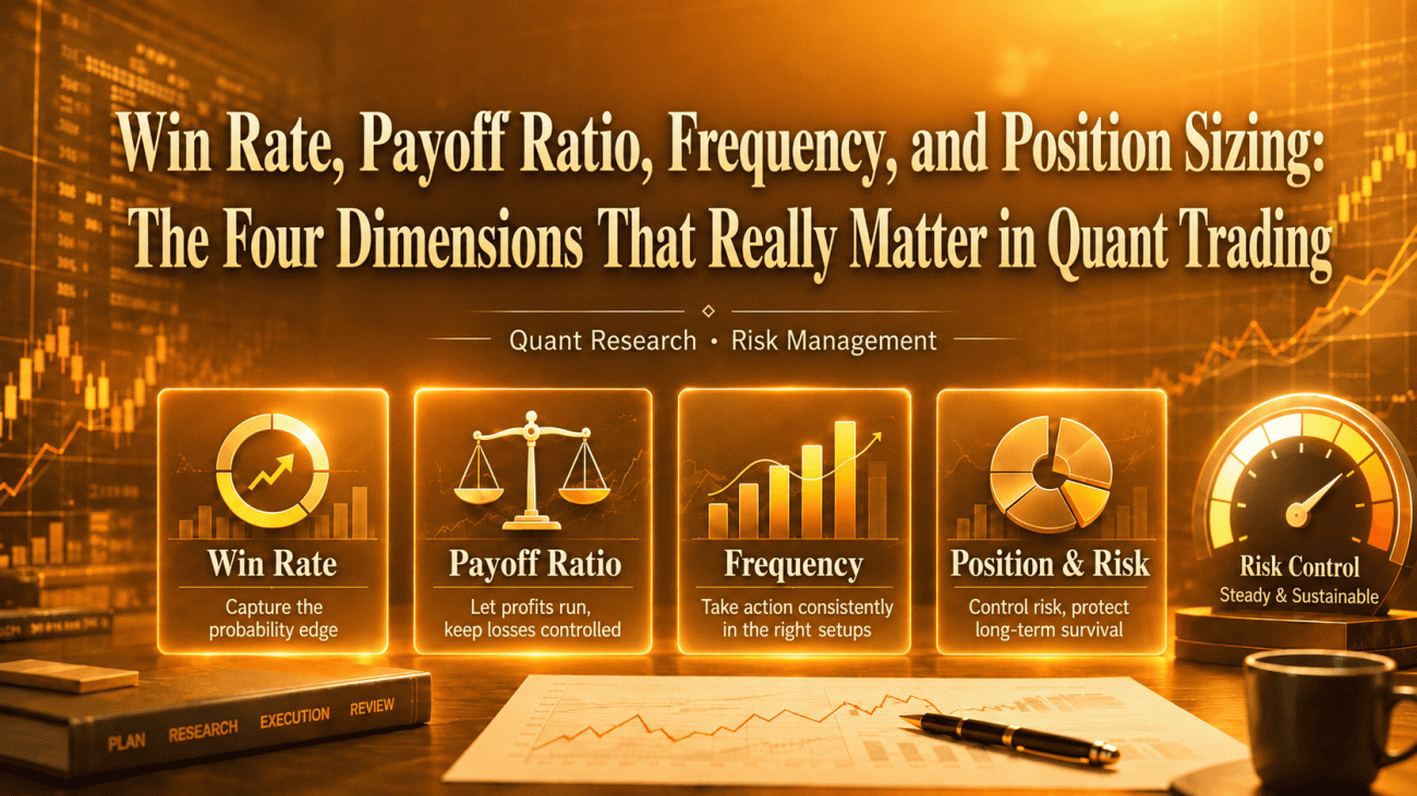
A quantitative strategy can be as complex as you like, but complexity alone does not tell you whether the strategy is worth trading.
Moving averages, RSI, machine-learning models, and even more sophisticated Agents all eventually come down to a few very simple questions:
How likely is the strategy to make money? How much does it make when it wins? How often do such opportunities appear? How much risk does it take each time?
In actual strategy operation, these correspond to the four dimensions that are most worth monitoring continuously:
win rate, payoff ratio, trading frequency, and position sizing.
These four dimensions do not describe every risk in a trading system, but they are extremely useful for answering one practical question:
How does a strategy's statistical edge ultimately translate into returns and drawdowns?
Using the cryptocurrency market and an FMZ strategy implementation as examples, this article focuses on how these four dimensions interact and how to turn them into live-trading monitoring metrics and risk constraints.
This article is for strategy research and software development purposes only and does not constitute investment advice.
1. Before Looking at Returns, Look at Net Expectancy per Trade
Let:
- the win rate be \(p\);
- the average winning trade be \(b\) times the average losing trade;
- commissions, slippage, and funding costs per trade equal \(c\) times the average loss.
If we normalize the average loss to one unit of risk, the net expectancy per trade can be written as:
\[ E = p \times b - (1-p) - c \]
This formula puts win rate, payoff ratio, and trading costs into the same framework.
For example, consider a BTC perpetual strategy with:
- a 42% win rate;
- a realized payoff ratio of 2.2:1;
- total trading costs of approximately 0.08 risk units per trade.
Then:
\[ E = 0.42 \times 2.2 - 0.58 - 0.08 = 0.264 \]
In other words, if these statistical characteristics can be maintained, each completed trade has an average net expectancy of approximately 0.264 risk units.
If the strategy plans to risk 0.5% of account equity per trade and produces 12 valid trades per month, then under the simplified assumptions of no compounding and no overlapping risk:
\[ 12 \times 0.264 \times 0.5\% = 1.584\% \]
This is not a return forecast.
What it really tells us is:
Win rate alone is meaningless, and payoff ratio alone is also meaningless. What matters is their combined expectancy after costs.
2. Win Rate and Payoff Ratio Must Be Evaluated Together
Among the four dimensions, this pair is probably the easiest to optimize incorrectly.
Many strategies can increase their win rate simply by changing the exit logic.
For example:
- taking profits earlier;
- widening stop losses;
- continuing to wait after a trade moves into a loss;
- averaging down to reduce the average entry price.
The result is often:
The win rate improves, but the average winner becomes smaller, the average loser becomes larger, and tail losses become more dangerous.
Consider a strategy with an 85% win rate, an average winner of 0.3R, and an average loser of 2.5R:
\[ 0.85 \times 0.3 - 0.15 \times 2.5 = -0.12R \]
It still has negative expectancy.
Conversely, a trend-following strategy may have a win rate of only around 30%–40%, yet a small number of large trends can compensate for many small losses.
So in live trading, it is not enough to save only one overall win-rate number. The following metrics are much more useful:
| Metric | Purpose |
|---|---|
| Rolling win rate | Detect whether the recent hit rate is changing |
| Average winner in R | Check whether profitable trades are still expanding enough |
| Average loser in R | Check whether stop losses are still working as intended |
| Expectancy per trade in R | Determine whether the strategy still has a statistical edge |
| Maximum single-trade loss in R | Detect tail risk and execution anomalies |
| MFE / MAE | Check whether take-profit and stop-loss rules match the actual price path |
Here, using R-multiples is especially useful because directly comparing USDT profit and loss can be misleading.
Define:
\[ R_{\text{realized}} = \frac{\text{Net PnL of the trade}} {\text{Planned risk amount at entry}} \]
For example:
A trade earns 100 USDT while the original planned risk was only 50 USDT. The result is therefore +2R.
Another trade earns 300 USDT but takes 500 USDT of planned risk. Its result is only +0.6R.
The second trade makes more money in absolute terms, but the first trade uses risk much more efficiently.
3. What Really Matters About Frequency Is the Number of Effective Opportunities
Frequency should not simply mean how many times a strategy trades per day or per month.
At a minimum, three different concepts should be distinguished:
signal frequency, order frequency, and completed-trade frequency.
A strategy may have only 20 genuine entry opportunities in a month while submitting, modifying, and canceling thousands of orders.
In that case, what increases may not be Alpha, but instead:
- commissions;
- bid-ask spread costs;
- slippage;
- API and order-state-management pressure;
- the probability of duplicate orders;
- market impact.
So a more important question than "How many trades are there?" is:
Does each additional trade still have enough net edge?
Suppose a minute-level strategy has an average gross edge of only 0.06% per trade, while the complete round-trip trading cost has already reached 0.05%.
Only 0.01% of edge remains.
A small deterioration in live execution may be enough to eliminate the positive expectancy entirely.
On the other hand, trading frequency cannot be reduced indefinitely either.
If a strategy produces only a few trades per year, then even if all of them are profitable, it is difficult to determine whether the strategy has a persistent long-term edge or whether that particular market regime simply happened to suit it.
Therefore, what should actually be optimized is neither "high frequency" nor "low frequency," but:
obtaining as many relatively independent positive-expectancy opportunities as possible while keeping trading costs manageable.
The word independent is important here.
If BTC, ETH, and SOL all generate long signals at the same time, that may look like three separate opportunities, but they may simply be three manifestations of the same crypto-market risk factor.
Opening three positions does not necessarily mean that you have obtained three independent sources of edge.
That is why a live system should also monitor:
- same-direction risk;
- cross-asset correlation;
- concentrated signals within the same time window;
- total notional exposure;
- total planned stop-loss risk.
4. Position Sizing Is Not Leverage; It Is Risk Budgeting
Position sizing is the variable among the four dimensions that actually converts a statistical edge into an account-level result.
The correct calculation sequence should be:
First decide the maximum amount you are willing to lose, then work backward to determine how much you should buy.
For example:
Account equity:
\[ 10{,}000\ \text{USDT} \]
Maximum planned risk per trade:
\[ 0.5\% \]
The risk budget is therefore:
\[ 10{,}000 \times 0.5\% = 50\ \text{USDT} \]
If the distance between the entry price and the stop-loss price is 2.5%, the approximate notional position size is:
\[ \frac{50}{2.5\%} = 2{,}000\ \text{USDT} \]
What actually determines the risk here is:
stop distance × notional position size.
Leverage mainly affects how much margin is occupied.
Of course, real markets also involve slippage, price gaps, insufficient liquidity, and liquidation risk. So "planning to lose 50 USDT" does not mean the actual loss will always be exactly 50 USDT.
This is why the system should record not only planned risk, but also:
\[ \frac{\text{Actual loss}}{\text{Planned risk}} \]
If a strategy is designed to lose no more than 1R per trade but live trading repeatedly produces losses of -1.5R or -2R, the first thing to inspect is not the signal logic but execution and risk control.
Portfolio Risk Must Also Be Controlled
Suppose the system simultaneously holds:
- a BTC long position;
- an ETH long position;
- a SOL long position.
Each trade has a planned risk of 0.5% of account equity.
Viewed independently, none of them appears large.
But if all three positions are fundamentally exposed to the same market direction, the real issue is what happens if all three stop losses are triggered together.
Therefore, position management should have at least three layers of risk limits:
| Risk Layer | Example |
|---|---|
| Per-trade risk | ≤ 0.5% |
| Cumulative same-direction risk | ≤ 1% |
| Total portfolio planned risk | ≤ 1.5% |
The exact numbers are not the point.
The important principle is:
It is not enough to limit the size of each individual trade. The system must also limit portfolio risk after correlated positions are stacked together.
5. The Four Dimensions Form a Profitability Chain
Putting the relationships above together, a simplified expectancy over a given period can be written as:
\[ E_{\text{period}} \approx N \times E_R \times r \]
where:
- \(E_R\): average net expectancy per trade, measured in R;
- \(N\): number of effective trading opportunities;
- \(r\): risk per trade as a percentage of account equity.
More generally, if the amount of risk differs from trade to trade, the relationship is closer to:
\[ E_{\text{period}} \approx \sum_i E_{R,i} \times r_i \]
This reveals an important point:
The four dimensions cannot be maximized independently.
Raising the profit target may increase the payoff ratio but reduce the win rate.
Relaxing signal conditions may increase trading frequency but reduce expectancy per trade.
Increasing position size can amplify returns, but it also amplifies drawdowns and model error.
Reducing the use of stop losses may improve the short-term win rate while transferring risk into a small number of extreme losses.
What really needs to be optimized is:
The overall structure formed by all four dimensions under trading-cost, drawdown, and execution constraints.
6. In FMZ, You Do Not Actually Need to Record Very Much
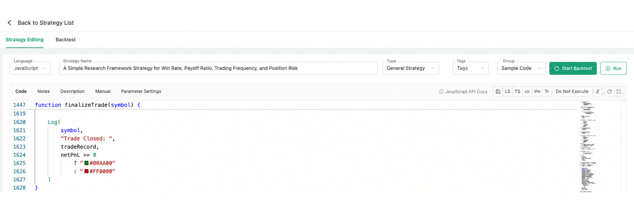
If the complete strategy source code already exists, there is little value in explaining GetTicker(), GetDepth(), or order-placement APIs one by one.
What the four-dimensional framework really needs is a unified trade record.
After every fully closed trade, at least the following data should be saved.
Group 1: Trade Identity and Time
| Field | Meaning | Purpose |
|---|---|---|
symbol | Trading instrument, such as BTC_USDT.swap | Separately evaluate BTC, ETH, or other instruments used by different strategy variants |
direction | Trade direction, such as long or short | Determine whether long-side and short-side performance differ materially |
entryTime | Time when the position was actually established | Analyze entry time, market regime, and trading frequency |
exitTime | Time when the position was fully closed | Combine with entry time to calculate holding period |
holdingTime | Duration from actual entry to complete exit | Detect meaningful changes in how long the strategy holds positions |
Group 2: Risk Baseline at Entry
| Field | Meaning | Purpose |
|---|---|---|
plannedRisk | Maximum planned risk amount at entry, for example 50 USDT | Baseline for calculating R-multiples and checking risk deviations |
equityAtEntry | Total account equity when the position is opened | Calculate how much account-level risk the trade actually consumes |
Group 3: Realized PnL and Trading Costs
| Field | Meaning | Purpose |
|---|---|---|
grossPnl | Trading PnL before additional costs | Measure how much gross profit the signal itself generated |
fee | Commissions generated by entry, exit, and other fills | Measure how much of the strategy edge is consumed by fees |
funding | Funding actually paid or received while holding a perpetual contract | Especially important for perpetual strategies with longer holding periods |
netPnl | Final net PnL after relevant cash costs | Used to calculate the true win rate, realized payoff ratio, and final expectancy |
slippage | Difference between theoretical and actual execution prices | Measure execution quality rather than signal quality alone |
Slippage is best stored separately as an execution-quality metric.
One definition requires particular care:
If grossPnl is already calculated from actual execution prices, the impact caused by execution prices deviating from theoretical prices has already entered the trading PnL.
Subtracting the same slippage from netPnl again may therefore result in double counting.
The system should clearly distinguish between:
cash costs and execution-attribution costs.
A More Robust Four-Dimensional Statistics Function
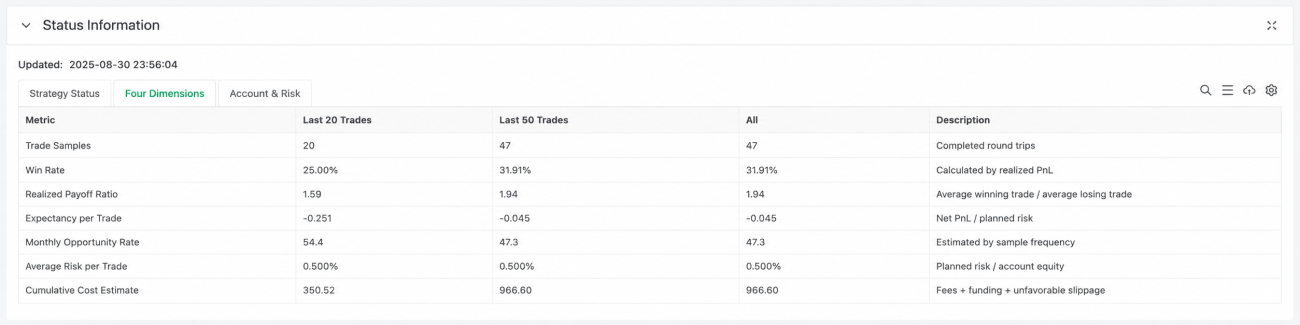
The principle is actually very simple.
Instead of reconstructing expectancy from the win rate and average win/loss, it is more robust to directly average the already standardized realizedR values of all trades.
javascript
function average(arr) {
if (!arr || arr.length === 0) {
return 0
}
return arr.reduce((sum, x) => sum + x, 0) / arr.length
}
function calcFourDimensions(trades) {
if (!trades || trades.length === 0) {
return null
}
const rs = trades.map(t => t.realizedR)
const wins = rs.filter(r => r > 0)
const losses = rs.filter(r => r < 0)
const avgWinR = wins.length ? average(wins) : 0
const avgLossR = losses.length ? Math.abs(average(losses)) : 0
return {
count: trades.length,
winRate:
wins.length / trades.length,
payoffRatio:
avgLossR > 0
? avgWinR / avgLossR
: null,
expectancyR:
average(rs),
avgRiskRate:
average(
trades
.filter(t => t.equityAtEntry > 0)
.map(t => t.plannedRisk / t.equityAtEntry)
)
}
}
The most important line is:
            javascript

            expectancyR = average(realizedR)
A breakeven trade is therefore simply 0. There is no need to artificially classify every trade as either a "win" or a "loss" before calculating expectancy.
It is also advisable to maintain at least two rolling windows, for example:
            text

            Most recent 20–30 trades
Most recent 100 trades
Then compare them with the historical backtest baseline.
Full-history statistics are useful only for answering:
"How has this strategy performed overall in the past?"
Rolling statistics are more useful for answering:
Is it still behaving the way it used to?
7. Testing the Four-Dimensional Framework With a Simple Strategy
There is no need to use a complicated signal model just to observe these four dimensions.
In fact, the Alpha component should be kept as simple as possible.
For example, we can use the following research strategy:
| Item | Rule |
|---|---|
| Market | BTC_USDT.swap / ETH_USDT.swap |
| Timeframe | 1 hour |
| Entry | A completed bar breaks out of the range formed by the previous 20 bars |
| Volatility | ATR(14) |
| Initial stop | 2 × ATR |
| Risk per trade | 0.5% of account equity |
| Same-direction risk | ≤ 1% |
| Total portfolio risk | ≤ 1.5% |
| Exit | Initial stop, reverse breakout, or trailing stop |
The strategy itself is not the Alpha this article is trying to prove.
It is only an experimental vehicle.
What we actually want to observe is:
What happens to the four dimensions after the signal passes through position sizing, costs, and execution?
For example, suppose the backtest shows:
            text

            Win rate               41%
Payoff ratio            2.4
Average trades/month    11
Average risk             0.5%
But the rolling live-trading window suddenly changes to:
            text

            Win rate                34%
Payoff ratio             1.3
Monthly trade frequency 27
Actual risk               0.8%
At this point, the issue is no longer simply "recent bad luck."
It may mean:
More false breakouts are reducing the win rate.
Earlier exits or shorter trends are reducing the payoff ratio.
Range-bound conditions are creating repeated entries and rapidly increasing trade frequency.
Slippage and execution anomalies are causing actual risk to exceed planned risk.
This is where a four-dimensional health check becomes genuinely useful.
8. Strategy Failure Should Be Divided Into Two Different Cases
One of the easiest mistakes to make in live trading is to confuse:
statistical strategy degradation with system execution failure.
They should be handled very differently.
Type 1: Statistical Degradation
For example:
- rolling expectancy continues to decline;
- win rate and payoff ratio deteriorate at the same time;
- effective opportunity frequency declines;
- costs consume a significantly larger share of gross profit;
- drawdown moves outside its historically normal range.
This type of situation usually still leaves room for observation.
Risk can be reduced first while the system continues collecting samples.
Type 2: System Failure
For example:
- abnormal market data;
- local position records do not match exchange positions;
- duplicate orders;
- order status cannot be confirmed;
- stop orders were not actually submitted or executed;
- actual risk repeatedly exceeds the system limit.
These problems do not require waiting for statistical significance.
The system should immediately stop adding new risk.
At that point, the question is no longer whether the Alpha is still valid, but whether the system can still execute correctly.
The Response Mechanism Can Be Compressed Into Three Levels
| Status | Typical Situation | Action |
|---|---|---|
| Normal / Observe | One metric deviates slightly while expectancy remains positive | Keep parameters unchanged and continue observing |
| Reduce Risk | Multiple statistical metrics deteriorate at the same time | Halve per-trade risk and reduce portfolio limits |
| Stop Opening New Positions | Expectancy remains negative or the execution system is abnormal | Stop adding new positions and investigate |
There is another important principle:
Do not immediately re-optimize parameters simply because the strategy has recently lost money.
Otherwise, it is easy to mistake normal random variation for strategy failure and then continuously chase the most recent market regime.
9. A Backtest Really Needs to Pass Only Three Gates
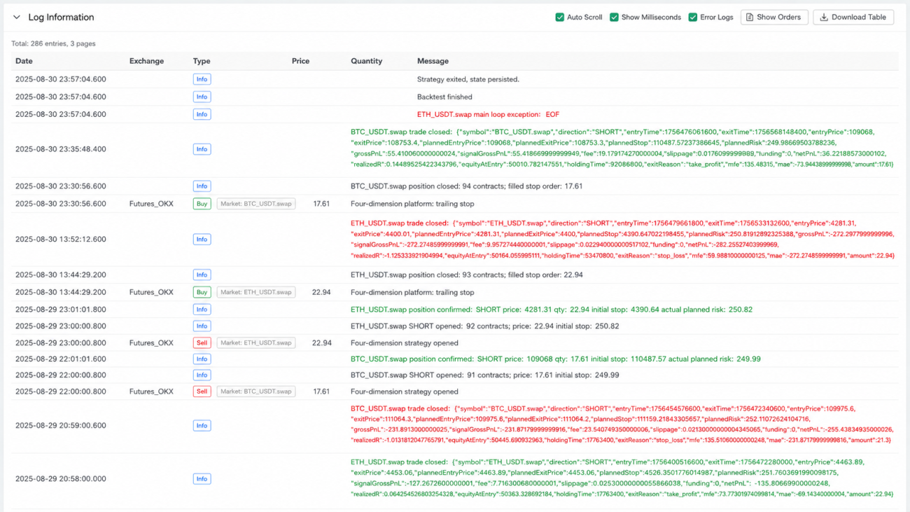
Instead of stacking up a large number of attractive-looking performance metrics, focus on three questions.
Gate 1: Does the Edge Still Exist After Costs?
After commissions, slippage, funding costs, and bid-ask spread are included, does the strategy still have positive expectancy?
If the strategy fails as soon as realistic trading costs are added, the original edge may have existed only because of idealized execution assumptions.
Gate 2: Does the Edge Exist Only for One Specific Parameter Set?
Change the breakout lookback from 20 bars to 18, 19, 21, and 22.
Change the ATR stop from 2 to 1.8 or 2.2.
Test a different time period.
Test BTC and ETH separately.
Then run the test again.
If only one extremely narrow parameter combination performs well, overfitting should be treated as a serious risk.
Gate 3: Can the Backtest Statistics Be Reproduced Under Real Execution?
During the small-capital live-trading stage, what actually needs to be verified is:
- whether
realizedRmatches expectations; - whether actual costs are close to the assumptions;
- whether order states are reliable;
- whether stop-loss risk remains under control;
- whether trading frequency becomes abnormal;
- whether portfolio risk is calculated and controlled correctly.
The key at this stage is not how much money the strategy makes.
The real objective is to confirm:
Does the four-dimensional structure observed in the backtest still exist in the real market?
Conclusion
Quantitative trading is not a "price-guessing contest."
A strategy does not need to be right every time.
What really needs to be built is a stable profitability chain:
Signals with a statistical edge
↓
A reasonable realized payoff ratio
↓
Enough effective trading opportunities, but not too many
↓
Position sizing that can survive consecutive losses and model error
Win rate tells us how often we make money.
Payoff ratio tells us how many losing trades one winning trade can cover.
Frequency determines whether the statistical edge can be realized within a finite amount of time, while also determining whether trading costs will consume that edge.
Position sizing determines whether the account can survive long enough for the edge to materialize.
The code simply keeps executing these rules consistently.
A mature quantitative trading system should always know three things:
- How much am I prepared to lose on this trade at most?
- Why might this strategy make money over the long run?
- Under what conditions should the system stop taking additional risk?
Complete FMZ strategy framework: Strategy Source Code
This strategy is for quantitative research and software development purposes only and does not constitute investment advice.
- 1