

SK Hynix has recently put the word “arbitrage” back in the spotlight.
With stock perpetual contracts going live, instruments such as SK Hynix and Samsung Electronics—which previously traded only through the KRX order book—gained an additional USDT-margined exposure channel with continuous 24-hour quotes. Public information shows that Binance listed SKHYNIXUSDT, SAMSUNGUSDT, and HYUNDAIUSDT on June 2, 2026. An industry report published in July noted that, during certain periods, the basis between SK Hynix’s Korean cash-market closing price and the Binance contract reached 3%–5%, while contract price differences across crypto platforms also exceeded 2% at one point. Once those spreads appeared on the screen, quantitative teams naturally rushed in. But after walking through that route myself, I did not ultimately trade it. Instead, I chose a quieter combination whose three legs could all be executed in the same account: EWY, Samsung Electronics, and SK Hynix.
This article explains the logic of the strategy: why I gave up on the cross-market basis trade, what makes the relationship among these three instruments potentially tradable, what the regression equation is doing, why the residual—not the price—is the actual trading object, how position ratios are determined, which data conditions must cause the strategy to refuse trading, and what is still missing before the current version can be considered suitable for live deployment. The strategy has been running in simulation on the FMZ Quant platform, and the source code is provided at the end.
1. The Basis Everyone Is Talking About—and the Timing Mismatch Behind It
The first point to clarify is a common wording error: listing stock perpetual contracts did not extend the trading hours of SK Hynix’s cash shares.
After the KRX closes, the underlying stock remains frozen at its final traded price, while the perpetual contract that references it continues to quote and absorb overnight macro data, movements in the Philadelphia Semiconductor Index, and exchange-rate changes. The reference asset is frozen while the derivative continues to price new information. This timing mismatch is the main source of the recent basis.
For the same reason, the so-called “fair price” after the cash market closes is unobservable. A deviation in the perpetual contract may arise from two completely opposite causes:
- It may be pricing overnight information in advance → the cash market could move toward it at the next open, in which case trading convergence means catching a falling knife against the trend.
- It may simply have been pushed away from its anchor by thin liquidity → the cash-market open could pull it back, in which case a convergence trade may be valid.
These two situations look exactly the same in the order book. If you cannot distinguish between them and place a bet anyway, you are not trading convergence—you are taking the other side of a new round of price discovery for the market.
2. Why I Did Not Pursue Cross-Market Arbitrage
Even if we set aside the ambiguity in pricing, building the “Korean cash equity ↔ crypto perpetual” trade requires passing through every one of the following frictions:
| Friction | Why It Eats Into the Quoted Spread |
|---|---|
| Trading-hour mismatch | While Korean equities are closed, the cash leg can neither be opened nor closed, leaving the exposure naked overnight. |
| Settlement currency | One side is a KRW asset, while the other is quoted in USDT, introducing FX exposure and conversion costs. |
| Funding channels | The two sides use completely different account systems, deposit and withdrawal routes, and short-selling conditions; capital cannot be transferred instantly. |
| Order-book depth | Newly listed contracts may have limited executable liquidity; the quoted spread is not the same as the executable spread. |
| Funding rates | The perpetual leg continuously generates carry during the holding period, and its direction may be unfavorable to the portfolio. |
| Trading restrictions | Price limits, temporary suspensions, and index rebalancing can make the “other leg” impossible to execute. |
A nominal 3% spread does not mean 3% will end up in your pocket. And the most visible crack is usually also the most crowded one.
So I changed the approach: keep the relative-value methodology, but place every leg in the same execution environment. This cannot eliminate strategy risk, but it can first remove several layers of engineering friction—accounts, funding channels, time zones, and settlement currencies—allowing the research to focus on the statistical relationship itself.
3. The Instruments: EWY and Its Two Heaviest Weights

Figure 1: EWY is like an asset basket containing multiple Korean companies, with Samsung Electronics and SK Hynix as its two heaviest weights. The regression attempts to use those two weights to explain the basket’s main movements, while the orange fluctuation represents the temporarily unexplained residual.
EWY is an ETF that tracks the South Korean equity market. According to the holdings disclosed by iShares on July 17, 2026:
| Component | Weight | Role in the Strategy |
|---|---|---|
| SK Hynix | ≈ 23.17% | Hedge leg 2 |
| Samsung Electronics | ≈ 21.72% | Hedge leg 1 |
| Others (Hyundai Motor, financial stocks, etc.) | ≈ 55% | One source of the residual |
Together, the two companies account for nearly 45% of the fund—enough to explain a large share of EWY’s directional movement, but far from enough to determine it completely. The remaining components, together with exchange rates, timing mismatches, capital flows, and the basis specific to each contract, create the deviations that may be traded.
The reason for choosing this combination is not that “the three curves look similar.” The deviation has an economic attribution: the two stocks are genuinely core holdings of the ETF. Because the statistical relationship is supported by the portfolio structure, it makes sense to discuss “convergence.” If you simply brute-force correlations across thousands of contracts, it is easy to find attractive but economically meaningless spurious relationships. Once the market regime changes, those relationships disappear.
The research question therefore becomes specific:
When EWY deviates from the “implied price” given by Samsung Electronics and SK Hynix, does that deviation tend to revert?
The strategy trades three USDT-margined linear contracts within the same account:
javascript
var SYMBOLS = "EWY_USDT.swap,SAMSUNG_USDT.swap,SKHYNIX_USDT.swap";
var LABELS = "EWY,Samsung Electronics,SK Hynix"; // The 1st is the target leg; the others are hedge legs
This must be stated clearly: it is not risk-free arbitrage. It is a relative-value trade that bets on the continuation of a statistical relationship.
4. The Model: Explaining the Basket with Two Weights
4.1 The Regression Equation—and Why It Uses Log Prices
            text

            ln(EWY) = c + β₁·ln(Samsung Electronics) + β₂·ln(SK Hynix) + ε
There are two practical reasons for using log prices rather than raw prices.
First, β becomes an elasticity coefficient. β₁ = 0.5 means that “when Samsung rises by 1%, EWY rises by 0.5%,” regardless of the absolute price levels of the three instruments. The resulting hedge ratios can be converted directly into notional amounts without multiplying by price ratios.
Second, the residual ε becomes a relative deviation. ε = 0.008 means that “EWY is approximately 0.8% more expensive than the value implied by the model.” It is a percentage. With a regression on raw prices, the residual is an absolute price difference whose units change as price levels change. It cannot be compared across time, and the standardized z-score loses its meaning.
4.2 Code Implementation
The mathematical core of the strategy is a single function. It returns not only β₁ and β₂, but also the full residual series for every K-line in the window—because the trading signal comes from the residual sequence, not from the coefficients themselves:
            javascript

            function regressSpread(lnTarget, lnRefs) {
    var k = lnRefs.length, n = lnTarget.length, dim = k + 1;
    var XtX = [], Xty = new Array(dim).fill(0);
    for (var i = 0; i < dim; i++) XtX.push(new Array(dim).fill(0));

    function col(j, t) { return j === 0 ? 1 : lnRefs[j - 1][t]; }

    // Accumulate the normal equations XᵀX and Xᵀy
    for (var t = 0; t < n; t++) {
        for (var i = 0; i < dim; i++) {
            Xty[i] += col(i, t) * lnTarget[t];
            for (var j = 0; j < dim; j++) XtX[i][j] += col(i, t) * col(j, t);
        }
    }
    var beta = solveLinearSystem(XtX, Xty);
    if (!beta) return null;

    // Reconstruct the residual bar by bar: actual value − model-implied value
    var resid = [];
    for (var t = 0; t < n; t++) {
        var pred = beta[0];
        for (var j = 0; j < k; j++) pred += beta[j + 1] * lnRefs[j][t];
        resid.push(lnTarget[t] - pred);
    }
    return { c: beta[0], betas: beta.slice(1), resid: resid };
}
solveLinearSystem() uses Gaussian elimination with partial pivoting. If the absolute value of a pivot is below 1e-12—meaning the two hedge legs are highly collinear and the normal equations are nearly singular—it returns null directly and invalidates the signal for that cycle. This is not numerical fussiness: Samsung and SK Hynix are both part of the Korean semiconductor sector, so collinearity is naturally high. A single ill-conditioned solution can push β to absurd magnitudes.
4.3 The Trading Object Is ε, Not Price
ε is “the part of EWY’s price that cannot be explained by the synchronized movement of Samsung and SK Hynix.” It may come from the ETF’s other constituents, such as Hyundai Motor and financial stocks, or from exchange rates, timing mismatches, funding rates, or liquidity noise.
This is the dividing line between this strategy and directional trading. We are not predicting whether the Korean stock market will rise or fall. We are betting only that “a short-term dislocation between the basket and its weights will converge.” The common movement of Samsung and SK Hynix is offset by the hedge legs, leaving only ε as the intended exposure.
The strategy runs a rolling regression on the most recent 480 fifteen-minute K-lines—approximately five trading days—and standardizes the latest residual:
            text

            z = (latest residual − mean residual over the window) / residual standard deviation over the window
There is a methodological flaw that must be acknowledged. The regression is fitted on the full sample within the window, and the latest residual participates in that fit. It is therefore naturally “pulled toward” the regression surface, systematically compressing the z-score. At the same time, the window rolls forward on every K-line, so β also changes. Strictly speaking, the residual sequence is not a set of comparable residuals generated by one fixed model. This is not fatal—rolling OLS is common in pairs trading—but it means the absolute z-score cannot be interpreted as a standard normal variable. Thresholds must be calibrated empirically; textbook conclusions such as “±2σ corresponds to 95%” cannot simply be applied.
5. The Signal: A Three-State Machine
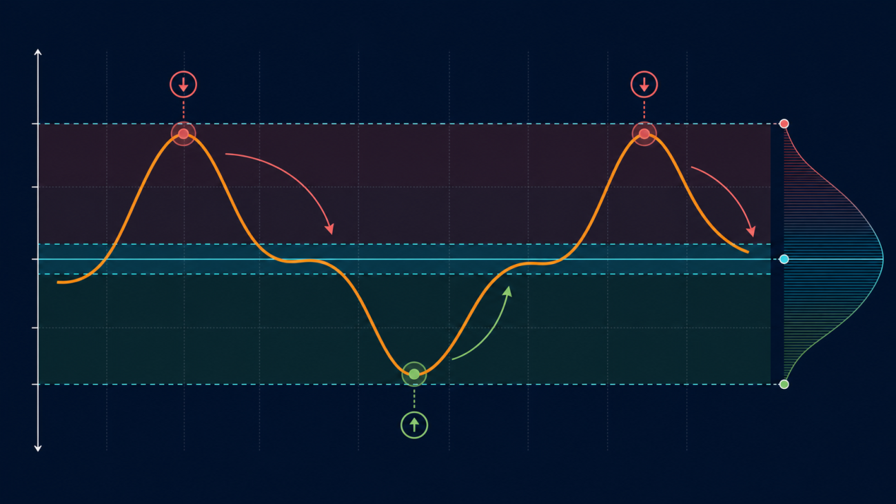
Figure 2: A spread position is opened when the residual enters the upper or lower extreme region and closed when it returns near the mean. The reversion arrows in the chart represent the trading hypothesis; they do not mean the residual is guaranteed to converge.
The signal is a small state machine. When flat, the strategy opens a position only after the entry threshold is crossed. Once a position is open, it does not keep adding just because z remains on the same side. It waits for z to return inside the exit band or for the maximum holding period to be reached.
            javascript

            var state = _G('bh_state') || 'FLAT';
var holdHours = state !== 'FLAT' ? (now - entryTime) / 3600000 : 0;
var forceExit = state !== 'FLAT' && MAX_HOLD_HOURS > 0 && holdHours > MAX_HOLD_HOURS;

var newState = state;
if (state === 'FLAT') {
    if (zLatest > ENTRY_Z)       newState = 'SHORT_SPREAD';  // EWY expensive → short EWY, long both hedge legs
    else if (zLatest < -ENTRY_Z) newState = 'LONG_SPREAD';   // EWY cheap → long EWY, short both hedge legs
} else {
    if (forceExit) { newState = 'FLAT'; Log('⏰ Maximum holding time exceeded; forcing exit'); }
    else if (Math.abs(zLatest) < EXIT_Z) { newState = 'FLAT'; Log('✅ z has reverted into the exit band; closing positions'); }
}
| State | Trigger | Direction of the Three Legs |
|---|---|---|
FLAT | Initial state / \|z\| < 0.5 / holding period exceeds 48h | No position |
SHORT_SPREAD | z > 1.0 | Short EWY, long Samsung, long SK Hynix |
LONG_SPREAD | z < −1.0 | Long EWY, short Samsung, short SK Hynix |
The asymmetric entry and exit thresholds—1.0 and 0.5—are deliberate. If they were equal, z would oscillate near the threshold and repeatedly open and close positions, allowing fees to consume the entire profit. The 0.5 buffer ensures that every trade must complete at least half a standard deviation of reversion before the gain is realized.
This state machine contains two design trade-offs that need to be stated explicitly:
- There is no z-based stop-loss. If z continues to widen against the position—for example, z rises from 1.2 to 3 while holding
SHORT_SPREAD—the code neither adds to the position nor stops out. It waits only for|z| < 0.5or for the 48-hour timeout. This is the classic form of a mean-reversion strategy, and also the classic way such a strategy dies: once the relationship truly breaks, the loss has no upper bound. - The strategy does not reverse. If z crosses directly to −1.5 while holding
SHORT_SPREAD, theelsebranch checks only|z| < 0.5and the timeout. Neither condition is met, so the position remains unchanged until the 48-hour limit. This is an explicit behavioral boundary, not a bug, but it should be reassessed before live trading.
The purpose of MAX_HOLD_HOURS = 48 is precisely to prevent a short-term dislocation from turning into a long-term belief. In this version, it is the only hard mechanism for admitting that “the relationship may already have failed.”
6. Positioning: β Determines the Ratios
The easiest mistake in a three-leg strategy is to get the direction right but the ratio wrong.
6.1 Where the Hedge Ratios Come From
Suppose the signal says EWY is expensive and we short one unit of EWY notional. What risks is the portfolio exposed to? According to the regression equation, β₁ units of EWY’s movement come from Samsung and β₂ units come from SK Hynix. To offset those two common factors, we must simultaneously buy β₁ units of Samsung notional and β₂ units of SK Hynix notional.
In the code, it is this line:
            javascript

            var wr = -reg.betas[j] * wTarget;   // Direction and size of each hedge leg are determined inversely by β
The notional ratio of the three legs is therefore 1 : β₁ : β₂, after which the whole portfolio is normalized to the gross exposure budget:
            javascript

            var dir = state === 'SHORT_SPREAD' ? -1 : 1;
var wTarget = dir * 1.0;
var wRefs = [], gross = Math.abs(wTarget);
for (var j = 0; j < reg.betas.length; j++) {
    var wr = -reg.betas[j] * wTarget;
    wRefs.push(wr); gross += Math.abs(wr);
}
var scale = gross > 0 ? (GROSS_EXPOSURE / gross) : 0;   // Normalize Σ|w| to 0.7
weights[0] = wTarget * scale;
for (var j = 0; j < wRefs.length; j++) weights[j + 1] = wRefs[j] * scale;
The strategy then converts weights into order quantities using notional amount = weight × LEVERAGE × equity, with leverage set to 3×.
The goal of this step is not to make the portfolio incapable of losing money. It is to make the portfolio sensitive only to ε. Broad moves in Korean equities, semiconductor-sector co-movement, and USD/KRW fluctuations—the factors acting simultaneously on all three legs—are theoretically offset by the β-based ratios. What remains is the relative-value component we actually want to trade.
6.2 When Orders Are Actually Placed
β and the weights are recalculated in every loop, but the strategy does not rebalance every time. Rebalancing is triggered only in two situations:
            javascript

            // ① The direction of any leg flips
if ((sig.weights[i] >= 0) !== (lastWeights[i] >= 0) && (sig.weights[i] !== 0 || lastWeights[i] !== 0)) {
    needRebal = true; break;
}
// ② The absolute weight of any leg drifts by more than 20%
var lw = Math.abs(lastWeights[i]);
if (lw > 1e-9 && Math.abs(Math.abs(sig.weights[i]) - lw) / lw > DRIFT_THRESHOLD) {
    needRebal = true; break;
}
β drift is captured through condition ②: β changes → weights change → the 20% threshold is exceeded → the hedge is rebalanced. This throttling layer acknowledges that “small fluctuations in β are estimation noise, not information.” If every minor change triggered a rebalance, trading fees would drain the account before the residual had time to converge.
MIN_REBAL_USDT = 3 serves two roles. It is both the threshold below which “the deviation is too small to act on” and the closing switch on exit. After the state changes to FLAT, the weights of all three legs become zero, making their target notionals fall below 3 USDT; the rebalancing logic then closes all positions.
7. Data Hygiene: Conditions That Must Block Trading
Newly listed TradFi contracts have short histories, prices may freeze during market closures, and the hedge legs are highly collinear. A single abnormal price can push β and z to absurd levels, causing the system to believe it has found a once-in-a-century opportunity.
For that reason, the code places several hard gates before a signal can be formed. They do not create returns. Their only job is to refuse trading when the data is clearly unreliable:
            javascript

            // ① Price-freeze detection: a hedge leg barely changes over the entire window
//    (market closed / mark price frozen). This destabilizes the regression,
//    compresses residual standard deviation toward zero, and can explode z.
if (refMax - refMin < MIN_REF_LOGRANGE) {          // 1e-6
    Log('⚠️ ' + LABELS[j + 1] + ' price barely changed within the window (possibly closed/frozen); skipping this cycle');
    return null;
}

// ② Collinearity detection: the normal equations are nearly singular,
//    so Gaussian elimination returns null
var reg = regressSpread(lnTarget, lnRefs);
if (!reg) { Log('⚠️ Regression matrix is singular; skipping this cycle'); return null; }

// ③ Minimum residual standard deviation: a very small value means the regression
//    is unreliable and the z denominator will amplify noise into a signal
var sd = stdev(reg.resid);
if (!(sd > MIN_RESID_STD)) { return null; }        // 5e-4

// ④ z-value sanity cap: an extreme value is more likely to be bad data
//    than a genuine opportunity
if (!isFinite(zLatest) || Math.abs(zLatest) > Z_SANITY_CAP) {   // 15
    Log('⚠️ Abnormal z value (' + zLatest + '); treating it as a calculation fault and ignoring the signal');
    return null;
}
Gate ① and gate ③ address opposite ends of the same risk. When Korean equities are closed, the reference contracts may remain unchanged for a long period, compressing the residual standard deviation within the window toward zero. The denominator of z then approaches zero, and any tiny numerator is magnified into an astronomical value. A seemingly “once-in-a-lifetime” z = 40 may simply be the result of dividing by a number that should never have appeared. If such signals are not blocked, the first trigger may be enough to wipe out the account.
The full data chain is also aligned. alignData() takes the intersection of timestamps across the three K-line series, keeps only times for which all three instruments have closing prices, and requires at least 490 common K-lines before any calculation is allowed. If any leg contains a zero, negative, or non-numeric price, the entire cycle is invalidated.
All intermediate values are logged with the [DEBUG] prefix: latest close, the log-price range of every leg within the window, regression coefficients, residual mean and standard deviation, and the raw z-score. If z becomes abnormal, the logs reveal exactly which stage caused the problem, without guesswork.
8. Risk Boundaries
Apart from z-based exits and the 48-hour timeout, the only active risk control in the code is a per-leg emergency reduction. If an open leg experiences an adverse move of more than 6% between two checks, the strategy cuts that leg’s position by half.
            javascript

            var drop = pos.side === 'long' ? (last - cur) / last : (cur - last) / last;
if (drop >= EMERGENCY_DROP) {                    // 0.06
    Log('🚨 Emergency risk! [' + label + '][' + pos.side + '] adverse move:', _N(drop * 100, 2) + '%');
    // ... reduce the position by 50%
}
Three boundaries of this mechanism must be made clear:
① It evaluates each leg individually, not the portfolio. In a hedged portfolio, one leg falling by 6% may be completely normal if another leg rises at the same time and the portfolio’s net exposure remains unchanged. In that situation, the circuit breaker damages the hedge structure. After half of a hedge leg is removed, the remaining exposure is no longer the residual; it becomes naked directional risk. This is the part of the current version that most urgently needs to be changed.
② The reference price is updated conditionally. bh_lastCheckPrices is updated as a whole only when no leg triggers during the current cycle. Once a trigger occurs, the reference price remains unchanged, and the next cycle still compares against the old price. In a one-way market, this can cause repeated triggers and repeated halving. This is intentionally conservative, but it can make the reduction much more aggressive than expected.
③ It is an after-the-fact defense. The three legs cannot fill in the same microsecond at the same ideal price. Once the first leg fills, the other two legs still leave the portfolio exposed to the market. That is leg risk. The faster the market moves, the more likely execution error is to consume the small residual the strategy is trying to earn. A per-leg circuit breaker reduces exposure only after a loss has already occurred. It cannot replace a genuine three-leg execution-coordination mechanism.
9. Parameter Summary
| Parameter | Default | Meaning |
|---|---|---|
INIT_CAPITAL | 400 USDT | Initial capital |
K_PERIOD | 15 minutes | K-line period |
LOOKBACK | 480 bars | Regression and z-score window (approximately five trading days) |
ENTRY_Z | 1.0 | Entry threshold |
EXIT_Z | 0.5 | Exit threshold |
MAX_HOLD_HOURS | 48 | Forced-exit time limit |
DRIFT_THRESHOLD | 0.20 | Re-hedge only after the weight drifts beyond this ratio |
LEVERAGE | 3 | Leverage |
GROSS_EXPOSURE | 0.7 | Sum of the absolute weights of the three legs |
MIN_REBAL_USDT | 3 | Minimum rebalancing notional / exit-closing switch |
EMERGENCY_DROP | 0.06 | Per-leg circuit-breaker threshold |
EMERGENCY_REDUCE | 0.50 | Position-reduction ratio after the circuit breaker triggers |
Z_SANITY_CAP | 15 | z-score sanity cap |
MIN_RESID_STD | 5e-4 | Minimum residual standard deviation |
MIN_REF_LOGRANGE | 1e-6 | Price-freeze detection threshold for hedge legs |
POLL_MS | 60 seconds | Main-loop polling interval |
⚠️ In the source code, the comment for
POLL_MSsays “5 minutes,” but the actual value is1 * 60 * 1000—one minute. Polling once per minute while using 15-minute K-lines means the same unfinished bar is recalculated repeatedly. As a result,DRIFT_THRESHOLDcarries a heavier throttling responsibility than originally intended. The implementation and the comment should be made consistent before live trading.
10. Two Days of Simulation—and What It Cannot Prove
The prototype ran in simulation on FMZ Quant with initial capital of 400 USDT. After two days of testing, the account recorded a certain amount of positive return.
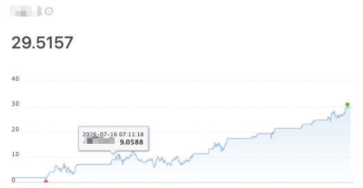
This is enough to justify continued research, but nowhere near enough to prove profitability:
- The sample is too short. Two days may cover only one market regime, or perhaps just one conveniently successful convergence. With a maximum holding period of 48 hours, the sample contains very few complete trade cycles.
- Simulated execution is friendlier than the real market. Orders are filled immediately and in full at the latest price, with no fees, no slippage, and no simulation of queue priority or partial fills. Three-leg strategies are especially sensitive to exactly these issues.
- Funding rates are not modeled at all. Funding rates across the three legs will not be identical. A long-short portfolio generates additional carry P&L that does not automatically cancel. The longer the holding period, the larger this bias becomes.
- Leg risk is not included. In the simulation, all three legs fill “simultaneously.” Real execution does not work that way.
The correct interpretation of the positive return at this stage is simply this: the workflow runs end to end, no abnormal circuit breaker was triggered, and z and β remained within reasonable ranges. Nothing more.
11. What the Current Version Does Not Implement
The difference between “the formula runs” and “capital can be entrusted to it” is the following checklist. None of these items is included in the current code, and every one of them must be completed before live deployment.
Statistical Validity
- No cointegration test. The code runs rolling OLS, but “running a regression” is not the same as “establishing cointegration.” An ADF or Engle–Granger test is needed to confirm that the residual is stationary. Otherwise, the supposed mean reversion may be nothing more than a visual illusion in a short sample.
- No half-life estimate. The residual has not been fitted to an OU process to estimate its reversion half-life.
MAX_HOLD_HOURS = 48is currently an arbitrary choice; it should instead be derived from the half-life. - No out-of-sample validation. There is no rolling walk-forward test and no parameter-stability analysis across market regimes. Neither
ENTRY_Z = 1.0norLOOKBACK = 480has been calibrated out of sample.
Costs and Execution
- Fees and slippage are not modeled. The average convergence amplitude of the residual must be reevaluated to determine whether any safety margin remains after costs.
- Funding-rate carry is not modeled. Funding rates for the three contracts must be tracked separately to determine whether the portfolio has a persistent carry bias toward one side.
- There is no three-leg execution-coordination mechanism. The system does not specify how to complete or unwind the whole portfolio within a limited time when legs fill separately, orders are rejected, execution is delayed, or fills are partial.
- Order precision is not aligned. Quantities are not rounded according to each contract’s
stepSizeand minimum notional requirement. - There is no trading calendar. The system does not identify KRX holidays, earnings windows, index rebalances, or other events during which β may change abruptly.
12. Where This Framework Can Be Extended
The same framework is not limited to the Korean market:
- Index vs. a basket of heavily weighted sectors: short-term deviations between the S&P 500 and several high-weight sector ETFs.
- Rotation among market leaders: relative dislocations between leaders and followers within the “Magnificent Seven.”
- Sector ETF vs. core constituents: constructing an implied value for an ETF from several of its largest holdings.
The model also does not have to remain a three-leg structure. The instrument pool can be expanded into “one target plus multiple explanatory factors.” But a larger portfolio is not automatically more sophisticated. Every additional leg introduces another order book, another fill process, another funding rate, and another failure point. Execution error on every leg directly erodes the small residual the strategy is trying to capture.
A genuinely tradable portfolio should satisfy all three conditions at the same time:
- The economic relationship makes sense—the deviation has an explanation and is not spurious correlation.
- The statistical relationship survives out-of-sample testing—it is not a coincidence in a short sample.
- Execution costs do not consume the expected return—net, not gross.
If even one is missing, the idea is research material, not a tradable opportunity.
Conclusion
The SK Hynix basis reminded the market that new trading vehicles create new price fractures. But arbitrage opportunities do not exist only in the most crowded fracture. Indices and constituents, ETFs and baskets of leading stocks, and leaders and followers within the same theme can all temporarily lose synchronization.
Formulas describe the deviation, tools discover and execute it, and risk controls give us a chance to survive until the next deviation appears. As for the small simulated profit in front of us, the right response is not celebration. It should be treated as the starting point for the next optimization checklist.
References
- Binance Academy: How to Trade SK Hynix (SKHY) on Binance
- ChainCatcher: Report on the Current Development Status of the Stock Perpetual Contract Market (July 2026)
- iShares: EWY Fund Information and Latest Holdings
Risk Notice: The content of this article is provided solely as a record of strategy research and simulated testing. It does not constitute investment advice. Statistical arbitrage is not risk-free arbitrage. Historical relationships, simulation results, and short-term returns do not guarantee future performance. The strategy runs in simulation mode by default. Complete every validation item listed above before switching to live trading.
Strategy source code: Three-Leg Pairs Statistical Arbitrage Strategy
- 1