Thinking about high-frequency trading strategies (1)
Author: The grass, Created: 2023-08-03 16:14:16, Updated: 2023-12-08 16:37:21
The article discusses high-frequency trading strategies for digital currencies, including the source of profits (mainly from strong market fluctuations and exchange fees), hanging positions and position control, and the method of modeling the volume of transactions using the Pareto distribution. In addition, it refers to the back-testing of one-to-one transactions and the best hanging order data provided by Binance, and plans to discuss other issues of high-frequency trading strategies in depth in subsequent articles.
I've written two articles before about high-frequency trading in digital currencies.High frequency strategies for digital currencies, 5 bands 80 times the power of high-frequency tacticsI'm planning to write a series of articles, introducing the idea of high-frequency trading from the beginning, hoping to be as brief as possible, but due to my own limited level, understanding of high-frequency trading is not in depth, this article is just throwing the dice, hopefully God is right.
High frequency source of profits
As mentioned in previous articles, high-frequency strategies are especially suitable for markets with very strong market fluctuations. Examine the price changes in a short period of time, consisting of overall trends and shocks. Of course, if we can accurately predict the changes in trends, we can make money, but this is also the most difficult. This article mainly introduces the high-frequency maker strategy, and will not address this issue.
Problems to be Solved
1.策略同时挂买单和卖单,第一个问题就是在哪里挂单。挂的离盘口越近,成交的概率越高,但在剧烈波动的行情中,瞬间成交的价格可能离盘口较远,挂的那太近没有能吃到足够的利润。挂的太远的单子成交概率又低。这是一个需要优化的问题。
2.控制仓位。为了控制风险,策略就不能长时间累计过多的仓位。可以通过控制挂单距离、挂单量、总仓位限制等办法解决。
In order to achieve the above purpose, it is necessary to model estimates of various aspects such as transaction probability probability, transaction profit, market estimation, etc. Many articles and papers on this subject can be found in keywords such as High-Frequency Trading, Orderbook etc. There are also many recommendations on the Internet, not here. It is also best to establish a reliable and fast feedback system.
Data needed
Binance provides transaction-by-transaction and best-in-class order dataDownloadedThe deep data needs to be downloaded in the whitelist using the API, and can also be collected on its own. The transaction data can be used for regression purposes. This article uses data from HOOKUSDT-aggTrades-2023-01-27.
from datetime import date,datetime
import time
import pandas as pd
import numpy as np
import matplotlib.pyplot as plt
%matplotlib inline
The following transactions were executed in cash:
- agg_trade_id: the id of the transaction,
- price: the transaction price
- quantity: the number of transactions
- first_trade_id: aggregate transaction may have several simultaneous transactions, statistically only one data item, which is the first transaction id
- last_trade_id: the id of the last transaction
- transact_time: time of completion of the transaction
- is_buyer_maker: transaction direction, True represents buyer-maker transaction, and buyer is the taker
You can see that there were 660,000 transaction data on the day and the transaction was very active.
trades = pd.read_csv('COMPUSDT-aggTrades-2023-07-02.csv')
trades
664475 rows × 7 columns
| agg_trade_id | price | quantity | first_trade_id | last_trade_id | transact_time | is_buyer_maker |
|---|---|---|---|---|---|---|
| 120719552 | 52.42 | 22.087 | 207862988 | 207862990 | 1688256004603 | False |
| 120719553 | 52.41 | 29.314 | 207862991 | 207863002 | 1688256004623 | True |
| 120719554 | 52.42 | 0.945 | 207863003 | 207863003 | 1688256004678 | False |
| 120719555 | 52.41 | 13.534 | 207863004 | 207863006 | 1688256004680 | True |
| … | … | … | … | … | … | … |
| 121384024 | 68.29 | 10.065 | 210364899 | 210364905 | 1688342399863 | False |
| 121384025 | 68.30 | 7.078 | 210364906 | 210364908 | 1688342399948 | False |
| 121384026 | 68.29 | 7.622 | 210364909 | 210364911 | 1688342399979 | True |
Modeling of single transaction
First, the data is processed, and the original trades are divided into the proactive transaction group for payment and the proactive transaction group for sales orders. The other data for the original aggregated transaction is one data at the same time and the same price in the same direction, there may be a volume of one proactive transaction of 100, if divided into several transactions with different prices, such as for 60 and 40 pieces, two data will be produced, affecting the estimate of the transaction volume.
trades['date'] = pd.to_datetime(trades['transact_time'], unit='ms')
trades.index = trades['date']
buy_trades = trades[trades['is_buyer_maker']==False].copy()
sell_trades = trades[trades['is_buyer_maker']==True].copy()
buy_trades = buy_trades.groupby('transact_time').agg({
    'agg_trade_id': 'last',
    'price': 'last',
    'quantity': 'sum',
    'first_trade_id': 'first',
    'last_trade_id': 'last',
    'is_buyer_maker': 'last',
    'date': 'last',
    'transact_time':'last'
})
sell_trades = sell_trades.groupby('transact_time').agg({
    'agg_trade_id': 'last',
    'price': 'last',
    'quantity': 'sum',
    'first_trade_id': 'first',
    'last_trade_id': 'last',
    'is_buyer_maker': 'last',
    'date': 'last',
    'transact_time':'last'
})
buy_trades['interval']=buy_trades['transact_time'] - buy_trades['transact_time'].shift()
sell_trades['interval']=sell_trades['transact_time'] - sell_trades['transact_time'].shift()
print(trades.shape[0] - (buy_trades.shape[0]+sell_trades.shape[0]))
146181
For example, if you draw a rectangle first, you can see that the long tail effect is very noticeable, with most of the data concentrated on the leftmost point, but also a small amount of large transactions distributed on the tail.
buy_trades['quantity'].plot.hist(bins=200,figsize=(10, 5));
)
为了观察方便,截掉尾部观察.可以看到成交量越大,出现频率越低,且减少的趋势更快。
buy_trades['quantity'][buy_trades['quantity']<200].plot.hist(bins=200,figsize=(10, 5));
)
The power-law distribution, also known as the Pareto distribution, is a form of probability distribution common in statistical physics and social science. In a power-law distribution, the probability of an event is proportional to some negative exponent of the event's size. The main characteristic of this distribution is that large events (i.e., events that are far from the mean) have a higher frequency of occurrence than would be expected in many other distributions.
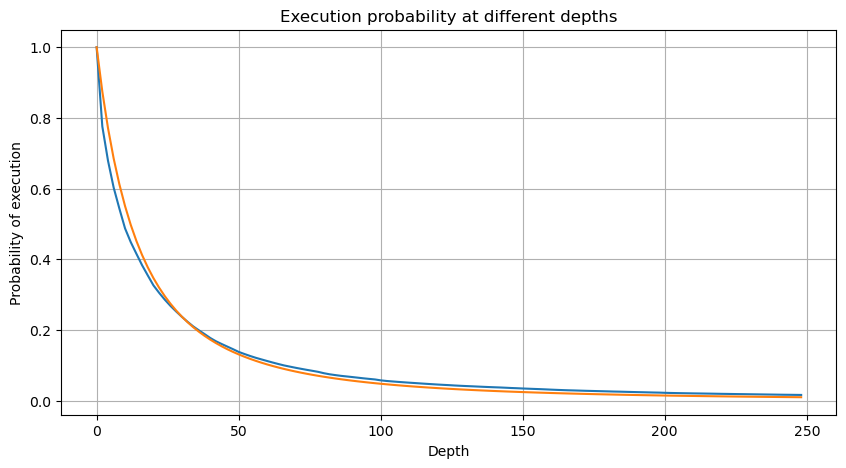
The following graph shows the probability of a transaction being completed at a value greater than a certain value, the blue line being the actual probability, the dashed line being the simulated probability, and without entangling the specific parameters, it can be seen that it does indeed satisfy the Pareto distribution. Since the probability of an order volume greater than 0 is 1, and in order to satisfy standardization, its distribution equation should take the following form:
)
where N is the standardized parameter. M is chosen as the average transaction, and alpha is chosen as 2.06. The estimate of the specific alpha can be calculated by taking the P value when D=N. Specifically: alpha = log (P (d) > M (l) /log (l)).
depths = range(0, 250, 2)
probabilities = np.array([np.mean(buy_trades['quantity'] > depth) for depth in depths])
alpha = np.log(np.mean(buy_trades['quantity'] > mean_quantity))/np.log(2)
mean_quantity = buy_trades['quantity'].mean()
probabilities_s = np.array([(1+depth/mean_quantity)**alpha for depth in depths])

plt.figure(figsize=(10, 5))
plt.plot(depths, probabilities)
plt.plot(depths, probabilities_s)
plt.xlabel('Depth')
plt.ylabel('Probability of execution')
plt.title('Execution probability at different depths')
plt.grid(True)
plt.figure(figsize=(10, 5))
plt.grid(True)
plt.title('Diff')
plt.plot(depths, probabilities_s-probabilities);
)
But this estimate only looks like the difference between the simulated and the actual value we have plotted in the diagram above. The deviation is very large, even close to 10%, when the transaction is smaller. Different points can be selected to make the probability of this point more accurate by estimating the parameters, but the deviation problem cannot be solved. This is determined by the difference between the parity distribution and the actual distribution, and in order to get more accurate results, the equation of the parity distribution needs to be modified.
)
For the sake of brevity, here r = q/M represents a standardized transaction volume. Parameters can be estimated in the same way as above. The graph below shows that the maximum deviation after the correction is no more than 2%, which can theoretically be further corrected, but this precision is also sufficient.
depths = range(0, 250, 2)
probabilities = np.array([np.mean(buy_trades['quantity'] > depth) for depth in depths])
mean = buy_trades['quantity'].mean()
alpha = np.log(np.mean(buy_trades['quantity'] > mean))/np.log(2.05)
probabilities_s = np.array([(((1+20**(-depth/mean))*depth+mean)/mean)**alpha for depth in depths])

plt.figure(figsize=(10, 5))
plt.plot(depths, probabilities)
plt.plot(depths, probabilities_s)
plt.xlabel('Depth')
plt.ylabel('Probability of execution')
plt.title('Execution probability at different depths')
plt.grid(True)
plt.figure(figsize=(10, 5))
plt.grid(True)
plt.title('Diff')
plt.plot(depths, probabilities_s-probabilities);
)
With an estimation equation for the volume distribution, the probability of the equation is not a true probability but a conditional probability. This is when the question is answered, what is the probability that the next order will be greater than a certain value if it occurs? What is the probability that orders of different depths will be transacted (ideally, less strictly, theoretically the order book will have new orders and withdrawals, and queues of the same depth).
I'm almost done with this post, and there are still many questions to be answered, which the following series of articles will try to answer.
- Smiley curve for delta hedging of bitcoin options
- Thoughts on High-Frequency Trading Strategies (5)
- Thoughts on High-Frequency Trading Strategies (4)
- Thinking about high-frequency trading strategies (5)
- Thinking about high-frequency trading strategies (4)
- Thoughts on High-Frequency Trading Strategies (3)
- Thinking about high-frequency trading strategies (3)
- Thoughts on High-Frequency Trading Strategies (2)
- Thinking about high-frequency trading strategies (2)
- Thoughts on High-Frequency Trading Strategies (1)
- Futu Securities Configuration Description Document
- FMZ Quant Uniswap V3 Exchange Pool Liquidity Related Operations Guide (Part 1)
- FMZ Quantitative Uniswap V3 Exchange Pool Liquidity related operating manual (1)
Orc quantified 🐂🍺
fmzeroI'm going to kill you.
The grassThe csv is too big to download yourself.