Thoughts on High-Frequency Trading Strategies (1)

I have written two articles on high-frequency trading of digital currencies, namely “Digital Currency High-Frequency Strategy Detailed Introduction” and “Earn 80 Times in 5 Days, the Power of High-frequency Strategy”. However, these articles can only be considered as sharing experiences and provide a general overview. This time, I plan to write a series of articles to introduce the thought process behind high-frequency trading from scratch. I hope to keep it concise and clear, but due to my limited expertise, my understanding of high-frequency trading may not be very in-depth. This article should be seen as a starting point for discussion, and I welcome corrections and guidance from experts.

Source of High-Frequency Profits

In my previous articles, I mentioned that high-frequency strategies are particularly suitable for markets with extremely volatile fluctuations. The price changes of a trading instrument within a short period of time consist of overall trends and oscillations. While it is indeed profitable if we can accurately predict trend changes, this is also the most challenging aspect. In this article, I will primarily focus on high-frequency maker strategies and will not delve into trend prediction. In oscillating markets, by placing bid and ask orders strategically, if the frequency of executions is high enough and the profit margin is significant, it can cover potential losses caused by trends. In this way, profitability can be achieved without predicting market movements. Currently, exchanges provide rebates for maker trades, which are also a component of profits. The more competitive the market, the higher the proportion of rebates should be.

Problems to be Addressed

1. The first problem in implementing a strategy that places both buy and sell orders is determining where to place these orders. The closer the orders are placed to the market depth, the higher the probability of execution. However, in highly volatile market conditions, the price at which an order is instantly executed may be far from the market depth, resulting in insufficient profit. On the other hand, placing orders too far away reduces the probability of execution. This is an optimization problem that needs to be addressed.

2. Position control is crucial to manage risk. A strategy cannot accumulate excessive positions for extended periods. This can be addressed by controlling the distance and quantity of orders placed, as well as setting limits on overall positions.

To achieve the above objectives, modeling and estimation are required for various aspects such as execution probabilities, profit from executions, and market estimation. There are numerous articles and papers available on this topic, using keywords such as “High-Frequency Trading” and “Orderbook.” Many recommendations can also be found online, although further elaboration is beyond the scope of this article. Additionally, it is advisable to establish a reliable and fast backtesting system. Although high-frequency strategies can easily be validated through live trading, backtesting provides additional insights and helps reduce the cost of trial and error.

Required Data

Binance provides downloadable data for individual trades and best bid/ask orders. Depth data can be downloaded through their API by being whitelisted, or it can be collected manually. For backtesting purposes, aggregated trade data is sufficient. In this article, we will use the example of HOOKUSDT-aggTrades-2023-01-27 data.

In [1]:

from datetime import date,datetime
import time
import pandas as pd
import numpy as np
import matplotlib.pyplot as plt
%matplotlib inline

The individual trade data includes the followings:

1. agg_trade_id: The ID of the aggregated trade.
2. price: The price at which the trade was executed.
3. quantity: The quantity of the trade.
4. first_trade_id: In cases where multiple trades are aggregated, this represents the ID of the first trade.
5. last_trade_id: The ID of the last trade in the aggregation.
6. transact_time: The timestamp of the trade execution.
7. is_buyer_maker: Indicates the direction of the trade. “True” represents a buy order executed as a maker, while a sell order is executed as a taker.

It can be seen that there were 660,000 trades executed on that day, indicating a highly active market. The CSV file will be attached in the comments section.

In [4]:

trades = pd.read_csv('COMPUSDT-aggTrades-2023-07-02.csv')
trades

Out[4]: , , , , , , , , , , , , , , , , , , , , , , , , , , , , , , , , , , , , , , , , , , , , , , , , , , , , , , , , , , , , , , , , , , , , , , , , , , , , , , , , , , , , , , , , , , , , , , , , , , , , , , , , , , , , , , , , , , , , , , , , , , , , , , ,

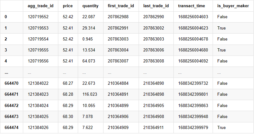
664475 rows × 7 columns

Modeling Individual Trade Amount

First, the data is processed by dividing the original trades into two groups: buy orders executed as makers and sell orders executed as takers. Additionally, the original aggregated trade data combines trades executed at the same time, at the same price, and in the same direction into a single data point. For example, if there is a single buy order with a volume of 100, it may be split into two trades with volumes of 60 and 40, respectively, if the prices are different. This can affect the estimation of buy order volumes. Therefore, it is necessary to aggregate the data again based on the transact_time. After this second aggregation, the data volume is reduced by 140,000 records.

In [6]:

trades['date'] = pd.to_datetime(trades['transact_time'], unit='ms')
trades.index = trades['date']
buy_trades = trades[trades['is_buyer_maker']==False].copy()
sell_trades = trades[trades['is_buyer_maker']==True].copy()
buy_trades = buy_trades.groupby('transact_time').agg({
    'agg_trade_id': 'last',
    'price': 'last',
    'quantity': 'sum',
    'first_trade_id': 'first',
    'last_trade_id': 'last',
    'is_buyer_maker': 'last',
    'date': 'last',
    'transact_time':'last'
})
sell_trades = sell_trades.groupby('transact_time').agg({
    'agg_trade_id': 'last',
    'price': 'last',
    'quantity': 'sum',
    'first_trade_id': 'first',
    'last_trade_id': 'last',
    'is_buyer_maker': 'last',
    'date': 'last',
    'transact_time':'last'
})
buy_trades['interval']=buy_trades['transact_time'] - buy_trades['transact_time'].shift()
sell_trades['interval']=sell_trades['transact_time'] - sell_trades['transact_time'].shift()

In [10]:

print(trades.shape[0] - (buy_trades.shape[0]+sell_trades.shape[0]))

Out [10]: 146181

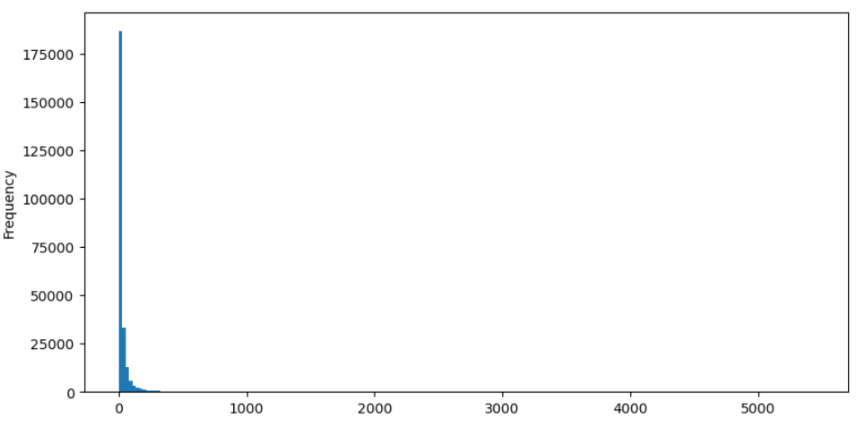
Take buy orders as an example, let’s first plot a histogram. It can be observed that there is a significant long-tail effect, with the majority of data concentrated towards the leftmost part of the histogram. However, there are also a few large trades distributed towards the tail end.

In [36]:

buy_trades['quantity'].plot.hist(bins=200,figsize=(10, 5));

Out [36]:

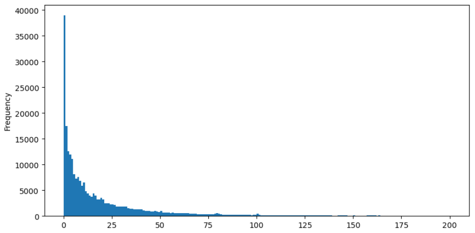
For easier observation, let’s trim the tail and analyze the data. It can be observed that as the trade amount increases, the frequency of occurrence decreases, and the rate of decrease becomes faster.

In [37]:

buy_trades['quantity'][buy_trades['quantity']<200].plot.hist(bins=200,figsize=(10, 5));

Out [37]:

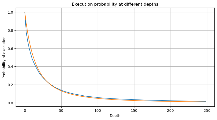
There have been numerous studies on the distribution of trade amounts. It has been found that trade amounts follow a power-law distribution, also known as a Pareto distribution, which is a common probability distribution in statistical physics and social sciences. In a power-law distribution, the probability of an event’s size (or frequency) is proportional to a negative exponent of that event’s size. The main characteristic of this distribution is that the frequency of large events (i.e., those far from the average) is higher than expected in many other distributions. This is precisely the characteristic of trade amount distribution. The form of the Pareto distribution is given by P(x) = Cx^(-α). Let’s empirically verify this.

The following graph represents the probability of trade amounts exceeding a certain value. The blue line represents the actual probability, while the orange line represents the simulated probability. Please note that we won’t go into the specific parameters at this point. It can be observed that the distribution indeed follows a Pareto distribution. Since the probability of trade amounts being greater than zero is 1, and in order to satisfy normalization, the distribution equation should be as follows:

Here, N is the parameter for normalization. We will choose the average trade amount, M, and set alpha to -2.06. The specific estimation of alpha can be obtained by calculating the P-value when D=N. Specifically, alpha = log(P(d>M))/log(2). The choice of different points may result in slight differences in the value of alpha.

In [55]:

depths = range(0, 250, 2)
probabilities = np.array([np.mean(buy_trades['quantity'] > depth) for depth in depths])
alpha = np.log(np.mean(buy_trades['quantity'] > mean_quantity))/np.log(2)
mean_quantity = buy_trades['quantity'].mean()
probabilities_s = np.array([(1+depth/mean_quantity)**alpha for depth in depths])

plt.figure(figsize=(10, 5))
plt.plot(depths, probabilities)
plt.plot(depths, probabilities_s)
plt.xlabel('Depth')
plt.ylabel('Probability of execution')
plt.title('Execution probability at different depths')
plt.grid(True)

Out[55]:

In [56]:

plt.figure(figsize=(10, 5))
plt.grid(True)
plt.title('Diff')
plt.plot(depths, probabilities_s-probabilities);

Out[56]:

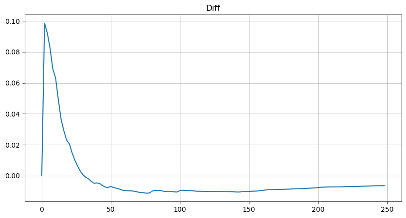
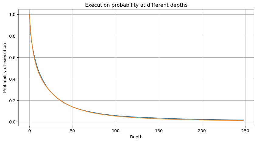
However, this estimation is only approximate, as shown in the graph where we plot the difference between the simulated and actual values. When the trade amount is small, the deviation is significant, even approaching 10%. Although selecting different points during parameter estimation may improve the accuracy of that specific point’s probability, it does not solve the deviation issue as a whole. This discrepancy arises from the difference between the power-law distribution and the actual distribution. To obtain more accurate results, the equation of the power-law distribution needs to be modified. The specific process is not elaborated here, but in summary, after a moment of insight, it is found that the actual equation should be as follows:

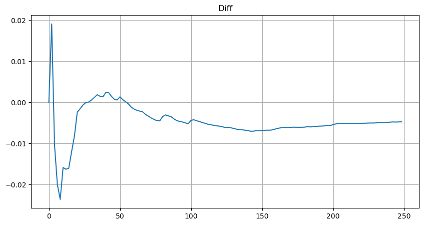
To simplify, let’s use r = q/M to represent the normalized trade amount. We can estimate the parameters using the same method as before. The following graph shows that after the modification, the maximum deviation is no more than 2%. In theory, further adjustments can be made, but this level of accuracy is already sufficient.

In [52]:

depths = range(0, 250, 2)
probabilities = np.array([np.mean(buy_trades['quantity'] > depth) for depth in depths])
mean = buy_trades['quantity'].mean()
alpha = np.log(np.mean(buy_trades['quantity'] > mean))/np.log(2.05)
probabilities_s = np.array([(((1+20**(-depth/mean))*depth+mean)/mean)**alpha for depth in depths])

plt.figure(figsize=(10, 5))
plt.plot(depths, probabilities)
plt.plot(depths, probabilities_s)
plt.xlabel('Depth')
plt.ylabel('Probability of execution')
plt.title('Execution probability at different depths')
plt.grid(True)

Out[52]:

In [53]:

plt.figure(figsize=(10, 5))
plt.grid(True)
plt.title('Diff')
plt.plot(depths, probabilities_s-probabilities);

Out[53]:

With the estimated equation for the trade amount distribution, it is important to note that the probabilities in the equation are not the actual probabilities, but conditional probabilities. At this point, we can answer the question: What is the probability that the next order will be greater than a certain value? We can also determine the probability of orders at different depths being executed (in an ideal scenario, without considering order additions, cancellations, and queueing at the same depth).

At this point, the length of the text is already quite long, and there are still many questions that need to be answered. The following series of articles will attempt to provide answers.