Thinking about high-frequency trading strategies (2)
Author: The grass, Created: 2023-08-04 16:14:27, Updated: 2023-09-19 09:08:17
The article mainly explores high-frequency trading strategies, with a focus on cumulative transaction modeling and price shocks. The article proposes a preliminary optimal hanging position model by analyzing single transactions, fixed-interval price shocks, and the effect of transactions on prices. The model attempts to find the optimal trading position based on an understanding of the volume of transactions and price shocks.
Accumulated traffic modeling
The previous post produced a probability expression for a single transaction that is larger than a certain value:
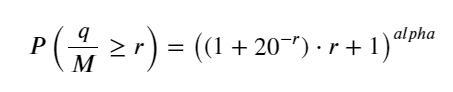
We are also concerned with the distribution of transactions over time, which should intuitively be related to the volume of transactions and order frequency per transaction.
from datetime import date,datetime
import time
import pandas as pd
import numpy as np
import matplotlib.pyplot as plt
%matplotlib inline
trades = pd.read_csv('HOOKUSDT-aggTrades-2023-01-27.csv')
trades['date'] = pd.to_datetime(trades['transact_time'], unit='ms')
trades.index = trades['date']
buy_trades = trades[trades['is_buyer_maker']==False].copy()
buy_trades = buy_trades.groupby('transact_time').agg({
    'agg_trade_id': 'last',
    'price': 'last',
    'quantity': 'sum',
    'first_trade_id': 'first',
    'last_trade_id': 'last',
    'is_buyer_maker': 'last',
    'date': 'last',
    'transact_time':'last'
})
buy_trades['interval']=buy_trades['transact_time'] - buy_trades['transact_time'].shift()
buy_trades.index = buy_trades['date']
The problem becomes a solved problem by combining transactions in 1s into a transaction volume, removing the non-transacted portion, and using the above distribution of transactions in 1s. This becomes a solved problem when the cycle is extended (relative to the frequency of transactions), and the error is found to increase, which is caused by the previous Pareto distribution correction. This means that when the cycle is extended, the more individual transactions are contained, the more transactions are combined and the closer they are to the cumulative Pareto distribution, this situation needs to be removed.
df_resampled = buy_trades['quantity'].resample('1S').sum()
df_resampled = df_resampled.to_frame(name='quantity')
df_resampled = df_resampled[df_resampled['quantity']>0]
buy_trades
| agg_trade_id | price | quantity | first_trade_id | last_trade_id | is_buyer_maker | date | transact_time | interval | diff | |
|---|---|---|---|---|---|---|---|---|---|---|
| 2023-01-27 00:00:00.161 | 1138369 | 2.901 | 54.3 | 3806199 | 3806201 | False | 2023-01-27 00:00:00.161 | 1674777600161 | NaN | 0.001 |
| 2023-01-27 00:00:04.140 | 1138370 | 2.901 | 291.3 | 3806202 | 3806203 | False | 2023-01-27 00:00:04.140 | 1674777604140 | 3979.0 | 0.000 |
| 2023-01-27 00:00:04.339 | 1138373 | 2.902 | 55.1 | 3806205 | 3806207 | False | 2023-01-27 00:00:04.339 | 1674777604339 | 199.0 | 0.001 |
| 2023-01-27 00:00:04.772 | 1138374 | 2.902 | 1032.7 | 3806208 | 3806223 | False | 2023-01-27 00:00:04.772 | 1674777604772 | 433.0 | 0.000 |
| 2023-01-27 00:00:05.562 | 1138375 | 2.901 | 3.5 | 3806224 | 3806224 | False | 2023-01-27 00:00:05.562 | 1674777605562 | 790.0 | 0.000 |
| … | … | … | … | … | … | … | … | … | … | … |
| 2023-01-27 23:59:57.739 | 1544370 | 3.572 | 394.8 | 5074645 | 5074651 | False | 2023-01-27 23:59:57.739 | 1674863997739 | 1224.0 | 0.002 |
| 2023-01-27 23:59:57.902 | 1544372 | 3.573 | 177.6 | 5074652 | 5074655 | False | 2023-01-27 23:59:57.902 | 1674863997902 | 163.0 | 0.001 |
| 2023-01-27 23:59:58.107 | 1544373 | 3.573 | 139.8 | 5074656 | 5074656 | False | 2023-01-27 23:59:58.107 | 1674863998107 | 205.0 | 0.000 |
| 2023-01-27 23:59:58.302 | 1544374 | 3.573 | 60.5 | 5074657 | 5074657 | False | 2023-01-27 23:59:58.302 | 1674863998302 | 195.0 | 0.000 |
| 2023-01-27 23:59:59.894 | 1544376 | 3.571 | 12.1 | 5074662 | 5074664 | False | 2023-01-27 23:59:59.894 | 1674863999894 | 1592.0 | 0.000 |
#1s内的累计分布
depths = np.array(range(0, 3000, 5))
probabilities = np.array([np.mean(df_resampled['quantity'] > depth) for depth in depths])
mean = df_resampled['quantity'].mean()
alpha = np.log(np.mean(df_resampled['quantity'] > mean))/np.log(2.05)
probabilities_s = np.array([((1+20**(-depth/mean))*depth/mean+1)**(alpha) for depth in depths])

plt.figure(figsize=(10, 5))
plt.plot(depths, probabilities)
plt.plot(depths, probabilities_s)
plt.xlabel('Depth')
plt.ylabel('Probability of execution')
plt.title('Execution probability at different depths')
plt.grid(True)
)
df_resampled = buy_trades['quantity'].resample('30S').sum()
df_resampled = df_resampled.to_frame(name='quantity')
df_resampled = df_resampled[df_resampled['quantity']>0]
depths = np.array(range(0, 12000, 20))
probabilities = np.array([np.mean(df_resampled['quantity'] > depth) for depth in depths])
mean = df_resampled['quantity'].mean()
alpha = np.log(np.mean(df_resampled['quantity'] > mean))/np.log(2.05)
probabilities_s = np.array([((1+20**(-depth/mean))*depth/mean+1)**(alpha) for depth in depths])
alpha = np.log(np.mean(df_resampled['quantity'] > mean))/np.log(2)
probabilities_s_2 = np.array([(depth/mean+1)**alpha for depth in depths]) # 无修正

plt.figure(figsize=(10, 5))
plt.plot(depths, probabilities,label='Probabilities (True)')
plt.plot(depths, probabilities_s, label='Probabilities (Simulation 1)')
plt.plot(depths, probabilities_s_2, label='Probabilities (Simulation 2)')
plt.xlabel('Depth')
plt.ylabel('Probability of execution')
plt.title('Execution probability at different depths')
plt.legend()
plt.grid(True)
)
Now for the distribution of different time-accumulated transactions, a general formula is summarized, and the distribution of single transactions is adjusted, without using separate statistics each time.
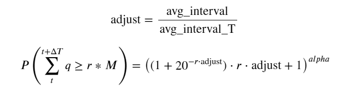
where avg_interval indicates the average interval between transactions, and avg_interval_T indicates the average interval between transactions that need to be estimated. This is somewhat circumvented. If we want to estimate transactions of 1s, we need to estimate the average interval between transactions that need to be included in 1s. If the probability of an order arriving is consistent with the Parsons distribution, it should be possible to directly estimate this, but the actual deviation is very large, which is not explained here.
Note that the probability of a transaction being completed in a certain time interval greater than a specific value here should differ significantly from the actual transaction probability of that location in the depth, because the longer the waiting time, the greater the probability of order book changes, and the transaction also causes a change in depth, so the probability of a transaction at the same depth location is changing in real time as the data is updated.
df_resampled = buy_trades['quantity'].resample('2S').sum()
df_resampled = df_resampled.to_frame(name='quantity')
df_resampled = df_resampled[df_resampled['quantity']>0]
depths = np.array(range(0, 6500, 10))
probabilities = np.array([np.mean(df_resampled['quantity'] > depth) for depth in depths])
mean = buy_trades['quantity'].mean()
adjust = buy_trades['interval'].mean() / 2620
alpha = np.log(np.mean(buy_trades['quantity'] > mean))/0.7178397931503168
probabilities_s = np.array([((1+20**(-depth*adjust/mean))*depth*adjust/mean+1)**(alpha) for depth in depths])

plt.figure(figsize=(10, 5))
plt.plot(depths, probabilities)
plt.plot(depths, probabilities_s)
plt.xlabel('Depth')
plt.ylabel('Probability of execution')
plt.title('Execution probability at different depths')
plt.grid(True)
)
The price of a single transaction shocks
Transaction data is a treasure trove, and there is a lot of data to mine. We should pay close attention to the impact of orders on prices, which affects the listing position of the strategy. Also based on transact_time aggregated data, calculate the difference between the last price and the first price, if there is only one order, the difference is 0.
The results showed that the proportion of non-impact was as high as 77%, the proportion of one tick was 16.5%, two ticks were 3.7%, three ticks were 1.2%, and four or more ticks were less than 1%. This is basically consistent with the characteristics of the exponential function, but the fit is not accurate.
The volume of transactions that caused the corresponding difference in price was calculated, removing too much distortion of the shock, and basically corresponding to a linear relationship, with about 1 tick for every 1000 volume. It can also be understood as a hanging volume of prices near each tray averaging about 1000.
diff_df = trades[trades['is_buyer_maker']==False].groupby('transact_time')['price'].agg(lambda x: abs(round(x.iloc[-1] - x.iloc[0],3)) if len(x) > 1 else 0)
buy_trades['diff'] = buy_trades['transact_time'].map(diff_df)
diff_counts = buy_trades['diff'].value_counts()
diff_counts[diff_counts>10]/diff_counts.sum()
0.000    0.769965
0.001    0.165527
0.002    0.037826
0.003    0.012546
0.004    0.005986
0.005    0.003173
0.006    0.001964
0.007    0.001036
0.008    0.000795
0.009    0.000474
0.010    0.000227
0.011    0.000187
0.012    0.000087
0.013    0.000080
Name: diff, dtype: float64
diff_group = buy_trades.groupby('diff').agg({
    'quantity': 'mean',
    'diff': 'last',
})
diff_group['quantity'][diff_group['diff']>0][diff_group['diff']<0.01].plot(figsize=(10,5),grid=True);
)
Fixed-range price shock
The difference here is that there will be a negative price shock within the statistic 2s, of course because only the payment is statistically counted here, the symmetrical position will be one tick larger. Continue to observe the relationship between the volume of transactions and the shock, only statistically greater than 0 results, the conclusion and the same for single orders, also an approximate linear relationship, each tick requires about 2000 quantities.
df_resampled = buy_trades.resample('2S').agg({
    'price': ['first', 'last', 'count'],
    'quantity': 'sum'
})
df_resampled['price_diff'] = round(df_resampled[('price', 'last')] - df_resampled[('price', 'first')],3)
df_resampled['price_diff'] = df_resampled['price_diff'].fillna(0)
result_df_raw = pd.DataFrame({
    'price_diff': df_resampled['price_diff'],
    'quantity_sum': df_resampled[('quantity', 'sum')],
    'data_count': df_resampled[('price', 'count')]
})
result_df = result_df_raw[result_df_raw['price_diff'] != 0]
result_df['price_diff'][abs(result_df['price_diff'])<0.016].value_counts().sort_index().plot.bar(figsize=(10,5));
)
result_df['price_diff'].value_counts()[result_df['price_diff'].value_counts()>30]
 0.001    7176
-0.001    3665
 0.002    3069
-0.002    1536
 0.003    1260
 0.004     692
-0.003     608
 0.005     391
-0.004     322
 0.006     259
-0.005     192
 0.007     146
-0.006     112
 0.008      82
 0.009      75
-0.007      75
-0.008      65
 0.010      51
 0.011      41
-0.010      31
Name: price_diff, dtype: int64
diff_group = result_df.groupby('price_diff').agg({ 'quantity_sum': 'mean'})
diff_group[(diff_group.index>0) & (diff_group.index<0.015)].plot(figsize=(10,5),grid=True);
)
The price shock of the transaction
The previous one asked for the required volume of a tick change, but it is not accurate, since it is based on the assumption that the shock has already occurred. Now look at the price shock caused by the tick change.
Here, the data is sampled in 1s, one step per 100 quantities, and the price changes within this range are calculated.
- When the order turnover is below 500, the expected price change is downward, which is expected, after all, there are also sell orders that affect the price.
- When the volume of transactions is low, the linear relationship corresponds, i.e. the larger the volume of transactions, the greater the price increase.
- The larger the transaction volume, the greater the price variation, which often represents a price breakout, and the price may rebound after the breakout, coupled with fixed interval sampling, causing data instability.
- The upper part of the scatter plot should be considered, i.e. the part where the volume of transactions corresponds to the price increase.
- For this transaction pair alone, give a rough version of the relationship between transaction volume and price changes:
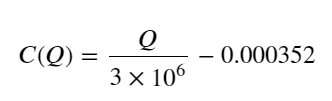
In this case, the C-value represents the change in price, and the Q-value represents the transaction volume.
df_resampled = buy_trades.resample('1S').agg({
    'price': ['first', 'last', 'count'],
    'quantity': 'sum'
})
df_resampled['price_diff'] = round(df_resampled[('price', 'last')] - df_resampled[('price', 'first')],3)
df_resampled['price_diff'] = df_resampled['price_diff'].fillna(0)
result_df_raw = pd.DataFrame({
    'price_diff': df_resampled['price_diff'],
    'quantity_sum': df_resampled[('quantity', 'sum')],
    'data_count': df_resampled[('price', 'count')]
})
result_df = result_df_raw[result_df_raw['price_diff'] != 0]
df = result_df.copy()
bins = np.arange(0, 30000, 100)  #
labels = [f'{i}-{i+100-1}' for i in bins[:-1]]
df.loc[:, 'quantity_group'] = pd.cut(df['quantity_sum'], bins=bins, labels=labels)
grouped = df.groupby('quantity_group')['price_diff'].mean()
grouped_df = pd.DataFrame(grouped).reset_index()
grouped_df['quantity_group_center'] = grouped_df['quantity_group'].apply(lambda x: (float(x.split('-')[0]) + float(x.split('-')[1])) / 2)

plt.figure(figsize=(10,5))
plt.scatter(grouped_df['quantity_group_center'], grouped_df['price_diff'],s=10)
plt.plot(grouped_df['quantity_group_center'], np.array(grouped_df['quantity_group_center'].values)/2e6-0.000352,color='red')
plt.xlabel('quantity_group_center')
plt.ylabel('average price_diff')
plt.title('Scatter plot of average price_diff by quantity_group')
plt.grid(True)
)
grouped_df.head(10)
| quantity_group | price_diff | quantity_group_center | |
|---|---|---|---|
| 0 | 0-199 | -0.000302 | 99.5 |
| 1 | 100-299 | -0.000124 | 199.5 |
| 2 | 200-399 | -0.000068 | 299.5 |
| 3 | 300-499 | -0.000017 | 399.5 |
| 4 | 400-599 | -0.000048 | 499.5 |
| 5 | 500-699 | 0.000098 | 599.5 |
| 6 | 600-799 | 0.000006 | 699.5 |
| 7 | 700-899 | 0.000261 | 799.5 |
| 8 | 800-999 | 0.000186 | 899.5 |
| 9 | 900-1099 | 0.000299 | 999.5 |
Initial most preferred single position
With a rough model of transaction volume modeling and transaction volume corresponding to price shocks, it seems possible to calculate the optimal hanging list position. You might want to make some assumptions and give an irresponsible optimal price position first.
- Assume that the price returns to its original value after the shock (this is of course unlikely and requires re-analysis of the price changes after the shock)
- Assume that the distribution of volume and frequency of orders during this time is as expected (this is also inaccurate, since the estimate is based on the value of a day, and there is a clear aggregation of transactions).
- Assume that there is only one sell order in the simulated time, and then break even.
- Assuming that after the order is placed, there are other payments that continue to push up the price, especially when the quantity is very low, this effect is ignored here, simply assuming that it will return.
First write a simple expected return, i.e. the probability that the cumulative payout is greater than Q in 1s, multiplied by the expected return (i.e. the price of the shock):
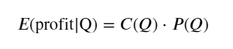
According to the image, the maximum expected return is around 2500, which is about 2.5 times the average transaction size. That is, the sell order should be hung at the 2500 position. It needs to be emphasized again that the transaction volume within the horizontal axis represents 1s, and cannot simply be equated with the depth position.
Summary
We found that the time-interval turnover distribution is a simple scaled-down of the single turnover distribution. We also made a simple expected return model based on price shocks and transaction probabilities, the results of which are in line with our expectations, if the turnover of the sold orders is small, predicting a decrease in prices, a certain amount is needed for profitability, and the larger the volume of transactions, the lower the probability, there is an optimal size in the middle, and the strategy is looking for a hanging position. Of course, this model is still too simple, I will continue to talk in depth in the next article.
#1s内的累计分布
df_resampled = buy_trades['quantity'].resample('1S').sum()
df_resampled = df_resampled.to_frame(name='quantity')
df_resampled = df_resampled[df_resampled['quantity']>0]

depths = np.array(range(0, 15000, 10))
mean = df_resampled['quantity'].mean()
alpha = np.log(np.mean(df_resampled['quantity'] > mean))/np.log(2.05)
probabilities_s = np.array([((1+20**(-depth/mean))*depth/mean+1)**(alpha) for depth in depths])
profit_s = np.array([depth/2e6-0.000352 for depth in depths])
plt.figure(figsize=(10, 5))
plt.plot(depths, probabilities_s*profit_s)
plt.xlabel('Q')
plt.ylabel('Excpet profit')
plt.grid(True)
)
- Smiley curve for delta hedging of bitcoin options
- Thoughts on High-Frequency Trading Strategies (5)
- Thoughts on High-Frequency Trading Strategies (4)
- Thinking about high-frequency trading strategies (5)
- Thinking about high-frequency trading strategies (4)
- Thoughts on High-Frequency Trading Strategies (3)
- Thinking about high-frequency trading strategies (3)
- Thoughts on High-Frequency Trading Strategies (2)
- Thoughts on High-Frequency Trading Strategies (1)
- Thinking about high-frequency trading strategies (1)
- Futu Securities Configuration Description Document
- FMZ Quant Uniswap V3 Exchange Pool Liquidity Related Operations Guide (Part 1)
- FMZ Quantitative Uniswap V3 Exchange Pool Liquidity related operating manual (1)
Orc quantified 🐂🍺