Thinking about high-frequency trading strategies (4)

The previous article showed why dynamic adjustment of parameters and how to evaluate estimates for good and bad is necessary by studying the order arrival interval. This article will focus on in-depth data, studying the mid-price (or fair-price, micro-price, etc.).

Deep data

Binance offers historical data downloads of the best bids, including best_bid_price: best bid_qty: best buy price, best_ask_price: best sell price, best_ask_qty: best sell price, transaction_time: time frame. This data does not include the second and deeper listings.

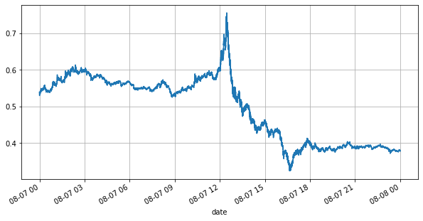
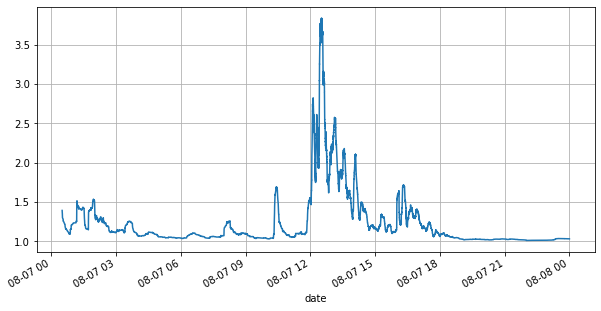
First of all, look at the market for the day, the big ups and downs, and the day's trading volume also changes significantly with the market fluctuations, especially the spread (the difference between a sell price and a buy price) very significantly indicates the volatility of the market.

from datetime import date,datetime
import time
import pandas as pd
import numpy as np
import matplotlib.pyplot as plt
%matplotlib inline

books = pd.read_csv('YGGUSDT-bookTicker-2023-08-07.csv')

tick_size = 0.0001

books['date'] = pd.to_datetime(books['transaction_time'], unit='ms')
books.index = books['date']

books['spread'] = round(books['best_ask_price'] - books['best_bid_price'],4)

books['best_bid_price'][::10].plot(figsize=(10,5),grid=True);

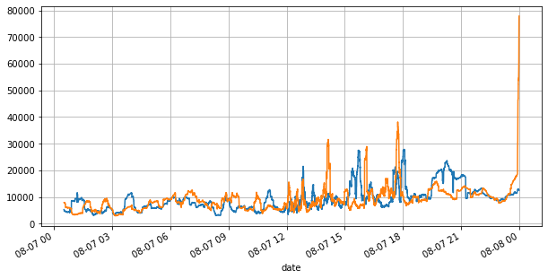
books['best_bid_qty'][::10].rolling(10000).mean().plot(figsize=(10,5),grid=True);
books['best_ask_qty'][::10].rolling(10000).mean().plot(figsize=(10,5),grid=True);

(books['spread'][::10]/tick_size).rolling(10000).mean().plot(figsize=(10,5),grid=True);

books['spread'].value_counts()[books['spread'].value_counts()>500]/books['spread'].value_counts().sum()

0.0001    0.799169
0.0002    0.102750
0.0003    0.042472
0.0004    0.022821
0.0005    0.012792
0.0006    0.007350
0.0007    0.004376
0.0008    0.002712
0.0009    0.001657
0.0010    0.001089
0.0011    0.000740
0.0012    0.000496
0.0013    0.000380
0.0014    0.000258
0.0015    0.000197
0.0016    0.000140
0.0017    0.000112
0.0018    0.000088
0.0019    0.000063
Name: spread, dtype: float64

Unbalanced offers

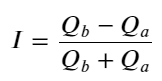
From the above, it can be seen that there is a large difference between the number of orders placed for purchase and the number of orders placed for sale most of the time, which is a strong predictor of the short-term market. The reason for this is the same as the reason for the small number of orders mentioned in the previous article. If one side of the order is significantly smaller than the other side, assuming that the volume of the next active buy and sell order is close, the small side of the order is more likely to be eaten, thus driving the price change.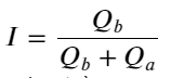Where Q_b represents the order quantity bid for (best_bid_qty) and Q_a represents the order quantity sold (best_ask_qty).

Definition of mid-price: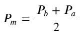

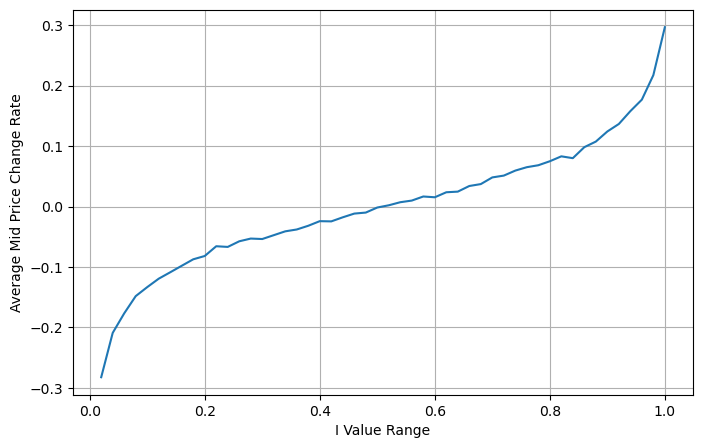
The following graph shows the relationship between the rate of change of the mid-price and the imbalance I at the following 1 interval, and the expected consistency, that the higher the I, the more likely the price is to rise, and the closer to 1, the greater the magnitude of the price change. In high-frequency trading, the purpose of introducing a mid-price is to better predict future price changes, i.e. the smaller the difference with the future price, the better the intermediate price is defined.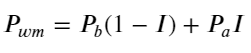

books['I'] = books['best_bid_qty'] / (books['best_bid_qty'] + books['best_ask_qty'])

books['mid_price'] = (books['best_ask_price'] + books['best_bid_price'])/2

bins = np.linspace(0, 1, 51)
books['I_bins'] = pd.cut(books['I'], bins, labels=bins[1:])
books['price_change'] = (books['mid_price'].pct_change()/tick_size).shift(-1)
avg_change = books.groupby('I_bins')['price_change'].mean()
plt.figure(figsize=(8,5))
plt.plot(avg_change)
plt.xlabel('I Value Range')
plt.ylabel('Average Mid Price Change Rate');
plt.grid(True)

books['weighted_mid_price'] = books['mid_price'] + books['spread']*books['I']/2
bins = np.linspace(-1, 1, 51)
books['I_bins'] = pd.cut(books['I'], bins, labels=bins[1:])
books['weighted_price_change'] = (books['weighted_mid_price'].pct_change()/tick_size).shift(-1)
avg_change = books.groupby('I_bins')['weighted_price_change'].mean()
plt.figure(figsize=(8,5))
plt.plot(avg_change)
plt.xlabel('I Value Range')
plt.ylabel('Weighted Average Mid Price Change Rate');
plt.grid(True)

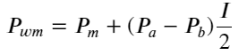
Adjusting the weighted average price

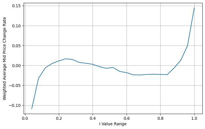
From the graph, the weighted mid-price variation is much smaller relative to the different I's, which indicates that the weighted mid-price is a better fit. However, there are still some rules, such as a large deviation near 0.2 and 0.8. This indicates that I can still contribute additional information. Since the weighted mid-price assumes that the price correction is completely linear with I, this is clearly not realistic, as can be seen from the graph above, the deviation is faster when I is close to 0 and 1, not a linear relationship.

To make it more intuitive, here I redefine I:

At this time:

Observing this form, it can be seen that the weighted median price is a correction to the mean median price, the coefficient of the correction is Spread, and the correction is about the function I, and the weighted mid-price simply assumes that the relationship is I/2 ⋅ This time the benefits of the adjusted distribution of I (−1,1) are reflected, I is about the symmetry of the origin, which provides us with a convenient relationship to find the fit of the function. Observing the graph, this function should satisfy the odd-second relation of I, which is consistent with the rapid growth of the two sides, and about the symmetry of the origin, it can also be observed that the value near the origin is linear, plus the function results 0 when the function is taken to be close to I0, and 0.5 when I is 1, so the function is conjectured as:

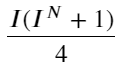
Here N is a positive even number, and after practical testing, N is better at 8; so far this article has proposed the corrected weighted median price:

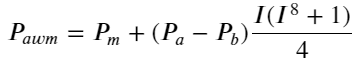
At this point, the prediction of the change in the median price is basically irrelevant to I. This result, although better than a simple weighted median price, is not applicable to the real world, just to give an idea. A 2017 article by S. Stoikov uses the method of Markov chains.Micro-PriceThis is the first time I have seen this blog, and I have given the code, which you can also look into.

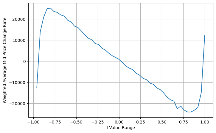
books['I'] = (books['best_bid_qty'] - books['best_ask_qty']) / (books['best_bid_qty'] + books['best_ask_qty'])

books['weighted_mid_price'] = books['mid_price'] + books['spread']*books['I']/2
bins = np.linspace(-1, 1, 51)
books['I_bins'] = pd.cut(books['I'], bins, labels=bins[1:])
books['weighted_price_change'] = (books['weighted_mid_price'].pct_change()/tick_size).shift(-1)
avg_change = books.groupby('I_bins')['weighted_price_change'].sum()
plt.figure(figsize=(8,5))
plt.plot(avg_change)
plt.xlabel('I Value Range')
plt.ylabel('Weighted Average Mid Price Change Rate');
plt.grid(True)

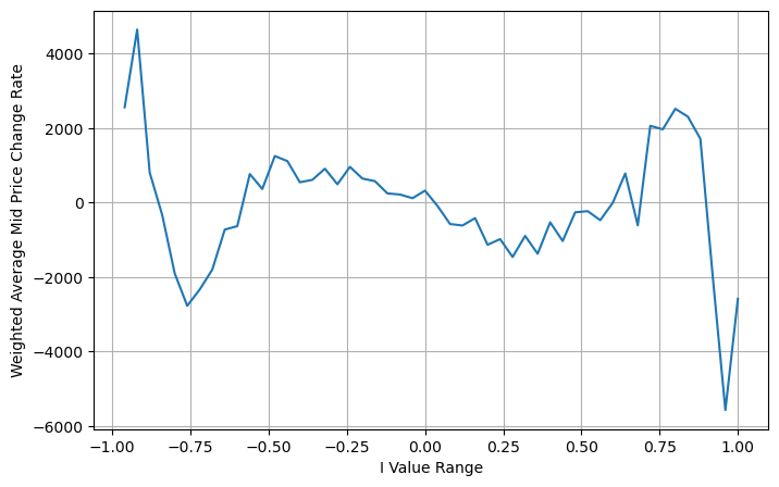
books['adjust_mid_price'] = books['mid_price'] + books['spread']*(books['I'])*(books['I']**8+1)/4
bins = np.linspace(-1, 1, 51)
books['I_bins'] = pd.cut(books['I'], bins, labels=bins[1:])
books['adjust_mid_price'] = (books['adjust_mid_price'].pct_change()/tick_size).shift(-1)
avg_change = books.groupby('I_bins')['adjust_mid_price'].sum()
plt.figure(figsize=(8,5))
plt.plot(avg_change)
plt.xlabel('I Value Range')
plt.ylabel('Weighted Average Mid Price Change Rate');
plt.grid(True)

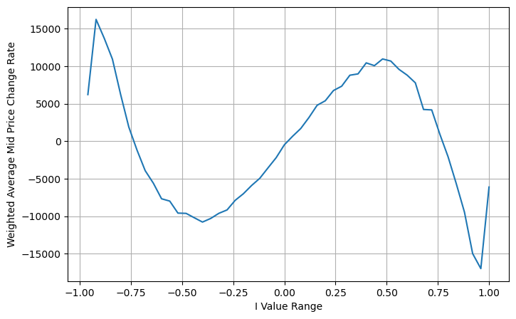
books['adjust_mid_price'] = books['mid_price'] + books['spread']*(books['I']**3)/2
bins = np.linspace(-1, 1, 51)
books['I_bins'] = pd.cut(books['I'], bins, labels=bins[1:])
books['adjust_mid_price'] = (books['adjust_mid_price'].pct_change()/tick_size).shift(-1)
avg_change = books.groupby('I_bins')['adjust_mid_price'].sum()
plt.figure(figsize=(8,5))
plt.plot(avg_change)
plt.xlabel('I Value Range')
plt.ylabel('Weighted Average Mid Price Change Rate');
plt.grid(True)

Summary

The intermediate price is very important for high-frequency strategies, it is a prediction of future short-term prices, so the intermediate price should be as accurate as possible. The intermediate prices described above are based on discounted data, which is because only one set of markets is used when analyzing. In the real market, the strategy is to use all data as much as possible, especially in the real market trades into exchanges, the prediction of the intermediate price should be checked by the actual transaction price.