Thinking about high-frequency trading strategies (5)

The previous article gave a preliminary introduction to the various methods of calculating the intermediate price and a revision of the intermediate price, which this article continues to delve into.

Required data

The order flow data and the depth data of ten disks are collected from the real disk, and the frequency of updates is 100 ms. The real disk only contains buy and sell per diskette data that is updated in real time, for brevity, temporarily not necessary. Given the data is too large, only 100,000 lines of depth data are kept, and the individual disks are also separated into separate columns.

from datetime import date,datetime
import time
import pandas as pd
import numpy as np
import matplotlib.pyplot as plt
import ast
%matplotlib inline

tick_size = 0.0001

trades = pd.read_csv('YGGUSDT_aggTrade.csv',names=['type','event_time', 'agg_trade_id','symbol', 'price', 'quantity', 'first_trade_id', 'last_trade_id',
       'transact_time', 'is_buyer_maker'])

trades = trades.groupby(['transact_time','is_buyer_maker']).agg({
    'transact_time':'last',
    'agg_trade_id': 'last',
    'price': 'first',
    'quantity': 'sum',
    'first_trade_id': 'first',
    'last_trade_id': 'last',
    'is_buyer_maker': 'last',
})

trades.index = pd.to_datetime(trades['transact_time'], unit='ms')
trades.index.rename('time', inplace=True)
trades['interval'] = trades['transact_time'] - trades['transact_time'].shift()

depths = pd.read_csv('YGGUSDT_depth.csv',names=['type','event_time', 'transact_time','symbol', 'u1', 'u2', 'u3', 'bids','asks'])

depths = depths.iloc[:100000]

depths['bids'] = depths['bids'].apply(ast.literal_eval).copy()
depths['asks'] = depths['asks'].apply(ast.literal_eval).copy()

def expand_bid(bid_data):
    expanded = {}
    for j, (price, quantity) in enumerate(bid_data):
        expanded[f'bid_{j}_price'] = float(price)
        expanded[f'bid_{j}_quantity'] = float(quantity)
    return pd.Series(expanded)
def expand_ask(ask_data):
    expanded = {}
    for j, (price, quantity) in enumerate(ask_data):
        expanded[f'ask_{j}_price'] = float(price)
        expanded[f'ask_{j}_quantity'] = float(quantity)
    return pd.Series(expanded)
# 应用到每一行，得到新的df
expanded_df_bid = depths['bids'].apply(expand_bid)
expanded_df_ask = depths['asks'].apply(expand_ask)
# 在原有df上进行扩展
depths = pd.concat([depths, expanded_df_bid, expanded_df_ask], axis=1)

depths.index = pd.to_datetime(depths['transact_time'], unit='ms')
depths.index.rename('time', inplace=True);

trades = trades[trades['transact_time'] < depths['transact_time'].iloc[-1]]

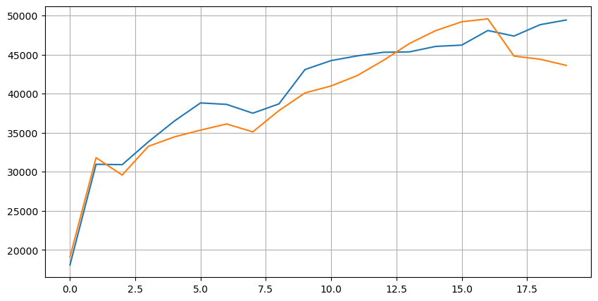
First of all, let's look at the distribution of these 20 file markets, which is in line with expectations, the further away from the listing, the more listings are generally listed, and the listings for purchase and sale are roughly symmetrical.

bid_mean_list = []
ask_mean_list = []
for i in range(20):
    bid_mean_list.append(round(depths[f'bid_{i}_quantity'].mean(),0))
    ask_mean_list.append(round(depths[f'ask_{i}_quantity'].mean(),0))
plt.figure(figsize=(10, 5))
plt.plot(bid_mean_list);
plt.plot(ask_mean_list);
plt.grid(True)

Combine the depth data with the transaction data to evaluate the accuracy of the forecast. This ensures that the transaction data is later than the depth data, and directly calculates the average error between the forecast value and the actual transaction price without taking into account the delay.

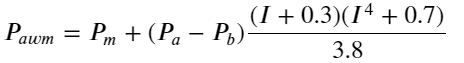
From the results, the error of buy/sell average mid_price is the largest, changed to weight_mid_price, the error is immediately much smaller, and slightly improved by adjusting the weighted mid-price. After yesterday's article was published, feedback was received with only I^3/2, which was checked here and found better results. Considering the following reasons, it should be the difference in frequency of occurrence of events, I is a low-probability event when close to -1 and 1, in order to correct these low probabilities, instead of making the prediction of high-frequency events less accurate, therefore, taking into account higher frequency events, I have adjusted the following:

The results are slightly better. As the previous article said, strategies should be predicted with more data, and with more depth and order transaction data, entanglement and leverage are already weak.

df = pd.merge_asof(trades, depths, on='transact_time', direction='backward')

df['spread'] = round(df['ask_0_price'] - df['bid_0_price'],4)
df['mid_price'] = (df['bid_0_price']+ df['ask_0_price']) / 2
df['I'] = (df['bid_0_quantity'] - df['ask_0_quantity']) / (df['bid_0_quantity'] + df['ask_0_quantity'])
df['weight_mid_price'] = df['mid_price'] + df['spread']*df['I']/2
df['adjust_mid_price'] = df['mid_price'] + df['spread']*(df['I'])*(df['I']**8+1)/4
df['adjust_mid_price_2'] = df['mid_price'] + df['spread']*df['I']*(df['I']**2+1)/4
df['adjust_mid_price_3'] = df['mid_price'] + df['spread']*df['I']**3/2
df['adjust_mid_price_4'] = df['mid_price'] + df['spread']*(df['I']+0.3)*(df['I']**4+0.7)/3.8

print('平均值     mid_price的误差：', ((df['price']-df['mid_price'])**2).sum())
print('挂单量加权 mid_price的误差：', ((df['price']-df['weight_mid_price'])**2).sum())
print('调整后的   mid_price的误差：', ((df['price']-df['adjust_mid_price'])**2).sum())
print('调整后的 mid_price_2的误差：', ((df['price']-df['adjust_mid_price_2'])**2).sum())
print('调整后的 mid_price_3的误差：', ((df['price']-df['adjust_mid_price_3'])**2).sum())
print('调整后的 mid_price_4的误差：', ((df['price']-df['adjust_mid_price_4'])**2).sum())

平均值     mid_price的误差： 0.0048751924999999845
挂单量加权 mid_price的误差： 0.0048373440193987035
调整后的   mid_price的误差： 0.004803654771638586
调整后的 mid_price_2的误差： 0.004808216498329721
调整后的 mid_price_3的误差： 0.004794984755260528
调整后的 mid_price_4的误差： 0.0047909595497071375

Consider the secondary depth.

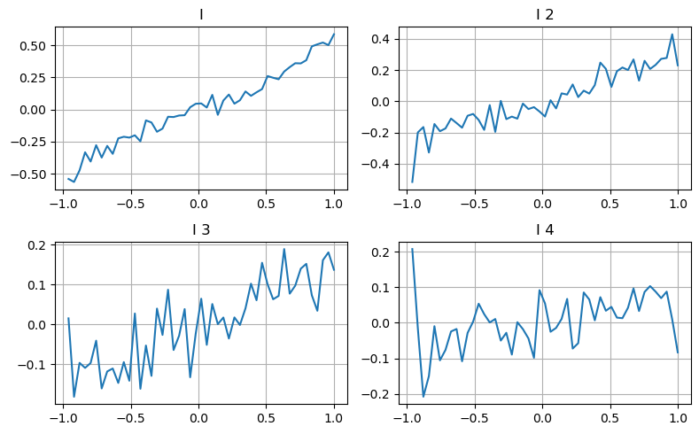
Here's an idea to look at the different range of values that affect a parameter, the change in the transaction price to measure the contribution of this parameter to the intermediate price. For example, the first depth graph shows that the more the transaction price increases, the more likely it is that the transaction price will change in the next direction, which indicates that I made a positive contribution.

The second movement was treated in the same way, and found that although the effect was slightly smaller than the first, it could not be ignored. The third movement also made a slight contribution, but the monotony was much worse, and the deeper depth had almost no reference value.

Depending on the degree of contribution, the imbalance parameters of the three grades are assigned different weights, and the actual check for different calculation methods further reduces the forecast error.

bins = np.linspace(-1, 1, 50)
df['change'] = (df['price'].pct_change().shift(-1))/tick_size
df['I_bins'] = pd.cut(df['I'], bins, labels=bins[1:])
df['I_2'] = (df['bid_1_quantity'] - df['ask_1_quantity']) / (df['bid_1_quantity'] + df['ask_1_quantity'])
df['I_2_bins'] = pd.cut(df['I_2'], bins, labels=bins[1:])
df['I_3'] = (df['bid_2_quantity'] - df['ask_2_quantity']) / (df['bid_2_quantity'] + df['ask_2_quantity'])
df['I_3_bins'] = pd.cut(df['I_3'], bins, labels=bins[1:])
df['I_4'] = (df['bid_3_quantity'] - df['ask_3_quantity']) / (df['bid_3_quantity'] + df['ask_3_quantity'])
df['I_4_bins'] = pd.cut(df['I_4'], bins, labels=bins[1:])
fig, axes = plt.subplots(nrows=2, ncols=2, figsize=(8, 5))


axes[0][0].plot(df.groupby('I_bins')['change'].mean())
axes[0][0].set_title('I')
axes[0][0].grid(True)

axes[0][1].plot(df.groupby('I_2_bins')['change'].mean())
axes[0][1].set_title('I 2')
axes[0][1].grid(True)

axes[1][0].plot(df.groupby('I_3_bins')['change'].mean())
axes[1][0].set_title('I 3')
axes[1][0].grid(True)

axes[1][1].plot(df.groupby('I_4_bins')['change'].mean())
axes[1][1].set_title('I 4')
axes[1][1].grid(True)
plt.tight_layout();

df['adjust_mid_price_4'] = df['mid_price'] + df['spread']*(df['I']+0.3)*(df['I']**4+0.7)/3.8
df['adjust_mid_price_5'] = df['mid_price'] + df['spread']*(0.7*df['I']+0.3*df['I_2'])/2
df['adjust_mid_price_6'] = df['mid_price'] + df['spread']*(0.7*df['I']+0.3*df['I_2'])**3/2
df['adjust_mid_price_7'] = df['mid_price'] + df['spread']*(0.7*df['I']+0.3*df['I_2']+0.3)*((0.7*df['I']+0.3*df['I_2'])**4+0.7)/3.8
df['adjust_mid_price_8'] = df['mid_price'] + df['spread']*(0.7*df['I']+0.2*df['I_2']+0.1*df['I_3']+0.3)*((0.7*df['I']+0.3*df['I_2']+0.1*df['I_3'])**4+0.7)/3.8

print('调整后的 mid_price_4的误差：', ((df['price']-df['adjust_mid_price_4'])**2).sum())
print('调整后的 mid_price_5的误差：', ((df['price']-df['adjust_mid_price_5'])**2).sum())
print('调整后的 mid_price_6的误差：', ((df['price']-df['adjust_mid_price_6'])**2).sum())
print('调整后的 mid_price_7的误差：', ((df['price']-df['adjust_mid_price_7'])**2).sum())
print('调整后的 mid_price_8的误差：', ((df['price']-df['adjust_mid_price_8'])**2).sum())

调整后的 mid_price_4的误差： 0.0047909595497071375
调整后的 mid_price_5的误差： 0.0047884350488318714
调整后的 mid_price_6的误差： 0.0047778319053133735
调整后的 mid_price_7的误差： 0.004773578540592192
调整后的 mid_price_8的误差： 0.004771415189297518

Consider the transaction data

The transaction data directly reflects the degree of over-space, after all, this is the choice of real gold and silver participation, while the cost of hanging orders is much lower, and even there are cases of deliberate hanging orders fraud. Therefore, forecasting intermediate prices, strategies should focus on the transaction data.

Taking into account the form, the average number of incoming orders is defined as unbalanced VI, Vb, and Vs respectively representing the average number of orders in the unit event of the buy and sell order.

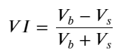
The results found that the number of arrivals in the short term is most significant for the prediction of price changes, when VI is between 0.1-0.9 and is negatively correlated with prices, while outside the range it is rapidly correlated with prices. This suggests that prices will return to equilibrium when the market is not extreme, dominated by shocks, and when extreme markets occur, such as when a large number of orders are overbought, which is when they leave the trend. Even if these low-probability situations are not taken into account, the simple assumption that the trend and VI satisfy a negative linear relationship, the prediction error difference for the intermediate price decreases significantly.

alpha=0.1

df['avg_buy_interval'] = None
df['avg_sell_interval'] = None
df.loc[df['is_buyer_maker'] == True, 'avg_buy_interval'] = df[df['is_buyer_maker'] == True]['transact_time'].diff().ewm(alpha=alpha).mean()
df.loc[df['is_buyer_maker'] == False, 'avg_sell_interval'] = df[df['is_buyer_maker'] == False]['transact_time'].diff().ewm(alpha=alpha).mean()

df['avg_buy_quantity'] = None
df['avg_sell_quantity'] = None
df.loc[df['is_buyer_maker'] == True, 'avg_buy_quantity'] = df[df['is_buyer_maker'] == True]['quantity'].ewm(alpha=alpha).mean()
df.loc[df['is_buyer_maker'] == False, 'avg_sell_quantity'] = df[df['is_buyer_maker'] == False]['quantity'].ewm(alpha=alpha).mean()

df['avg_buy_quantity'] = df['avg_buy_quantity'].fillna(method='ffill')
df['avg_sell_quantity'] = df['avg_sell_quantity'].fillna(method='ffill')
df['avg_buy_interval'] = df['avg_buy_interval'].fillna(method='ffill')
df['avg_sell_interval'] = df['avg_sell_interval'].fillna(method='ffill')

df['avg_buy_rate'] = 1000 / df['avg_buy_interval']
df['avg_sell_rate'] =1000 / df['avg_sell_interval']

df['avg_buy_volume'] = df['avg_buy_rate']*df['avg_buy_quantity']
df['avg_sell_volume'] = df['avg_sell_rate']*df['avg_sell_quantity']

df['I'] = (df['bid_0_quantity']- df['ask_0_quantity']) / (df['bid_0_quantity'] + df['ask_0_quantity'])
df['OI'] = (df['avg_buy_rate']-df['avg_sell_rate']) / (df['avg_buy_rate'] + df['avg_sell_rate'])
df['QI'] = (df['avg_buy_quantity']-df['avg_sell_quantity']) / (df['avg_buy_quantity'] + df['avg_sell_quantity'])
df['VI'] = (df['avg_buy_volume']-df['avg_sell_volume']) / (df['avg_buy_volume'] + df['avg_sell_volume'])

bins = np.linspace(-1, 1, 50)
df['VI_bins'] = pd.cut(df['VI'], bins, labels=bins[1:])
plt.plot(df.groupby('VI_bins')['change'].mean());
plt.grid(True)

df['adjust_mid_price'] = df['mid_price'] + df['spread']*df['I']/2
df['adjust_mid_price_9'] = df['mid_price'] + df['spread']*(-df['OI'])*2
df['adjust_mid_price_10'] = df['mid_price'] + df['spread']*(-df['VI'])*1.4

print('调整后的mid_price   的误差：', ((df['price']-df['adjust_mid_price'])**2).sum())
print('调整后的mid_price_9 的误差：', ((df['price']-df['adjust_mid_price_9'])**2).sum())
print('调整后的mid_price_10的误差：', ((df['price']-df['adjust_mid_price_10'])**2).sum())

调整后的mid_price   的误差： 0.0048373440193987035
调整后的mid_price_9 的误差： 0.004629586542840461
调整后的mid_price_10的误差： 0.004401790287167206

Integrated intermediate prices

Given that both the hanging order volume and the transaction data are helpful for forecasting the intermediate price, it is possible to combine the two parameters together, where the weighting is given relatively arbitrarily, without taking into account boundary conditions. In extreme cases, the forecasted intermediate price may not be between buy one and sell one, but as long as the error can be reduced, these details are not taken into account.

The error in the final forecast dropped from 0.00487 to 0.0043 at the beginning, and we can't go deeper here, there is a lot more to be mined in the middle price, after all, the forecast middle price is in the forecast price, you can try it yourself.

#注意VI需要延后一个使用
df['price_change'] = np.log(df['price']/df['price'].rolling(40).mean())
df['CI'] = -1.5*df['VI'].shift()+0.7*(0.7*df['I']+0.2*df['I_2']+0.1*df['I_3'])**3 + 150*df['price_change'].shift(1)

df['adjust_mid_price_11'] = df['mid_price'] + df['spread']*(df['CI'])
print('调整后的mid_price_11的误差：', ((df['price']-df['adjust_mid_price_11'])**2).sum())

调整后的mid_price_11的误差： 0.00421125960463469

Summary

This article combines in-depth data and transaction data, further improving the calculation of the intermediate price method, giving a method to measure accuracy, improving the accuracy of the prediction of price changes. On the whole, various parameters are not very strict, only for reference. There are more accurate intermediate prices, then the actual application of the intermediate price is re-measured.