In the previous article (((https://www.fmz.com/digest-topic/4187In this article, we introduce pairing trading strategies and demonstrate how to create and automate trading strategies using data and mathematical analysis.

The multi-space equilibrium equity strategy is a natural extension of the pairing trading strategy that applies to a basket of trading indices. It is particularly applicable to a wide variety of interconnected trading markets, such as the digital currency market and the commodity futures market.

Basic Principles

The multi-space balancing equity strategy is one that simultaneously trades a basket of stocks in both oversold and oversold. Like a pair of trades, it determines which stocks are cheap and which stocks are expensive. The difference is that the multi-space balancing equity strategy will line up all stocks in a pool of options to determine which stocks are relatively cheap or expensive.

Remember we said before that pairing is a market-neutral strategy? The same is true of the multi-head equity strategy, because the multi-head and empty-head equity positions ensure that the strategy will remain market-neutral (untouched by market fluctuations). The strategy is also statistically sound; by ranking an investment and holding multiple positions, you can take multiple positions on your ranking model, not just one.

What is the ranking scheme?

A ranking scheme is a model that prioritizes each indicator according to its expected performance. The factors can be value factors, technical indicators, pricing models, or a combination of all of the above. For example, you can use momentum indicators to rank a range of trend-tracking indicators: the indicator with the highest momentum is expected to continue to perform well and rank highest; the investment with the least momentum performs the worst and has the lowest return.

The success of this strategy lies almost entirely in the ranking scheme used, i.e. your ranking scheme is able to separate the high-performing investment indicators from the low-performing investment indicators to better realize the returns of the multi-empty investment indicator strategy.

How do you create a ranking scheme?

Once we have identified a ranking scheme, we obviously want to be able to profit from it. We do this by investing the same amount of money in the most ranked and lowest ranked investments. This ensures that the strategy will only make money proportionally to the quality of the ranking and will be "market neutral".

Suppose that you are ranking all of the m indices, have an investment of n dollars, and want to hold positions with a total of 2p (where m> 2p). If the index ranked 1 is expected to perform worst, then the index ranked m is expected to perform best:

• You're going to arrange the index in a position like 1,..., p, and you're going to make a blank 2/2p dollar index.

• You're going to arrange the index as: m-p,..., m, so you're going to do an index of n/2p dollars.

**Note: **Since the price of an investment indicator caused by a price jump will not always be evenly distributed n/2p, and certain investment indicators must be purchased in integers, there will be some imprecise algorithms that should be as close to this number as possible. For strategies running n = 100000 and p = 500, we see:

n/2p = 100000/1000 = 100

This creates a big problem for price scores greater than 100 (e.g. commodity futures market) because you can't open a position with a scoring price (the digital currency market doesn't exist). We mitigate this by reducing scoring price trading or increasing capital.

Let's take a hypothetical example.

• Inventors are building our research environment on a quantified platform.

First of all, in order for the work to proceed smoothly, we need to build our research environment, which we use in this article as an inventor quantification platform.FMZ.COMThe purpose of the project is to build a research environment, mainly for the convenient and fast API interfaces and well-wrapped Docker systems that can be used later on.

In the official name of the inventor's quantification platform, this Docker system is called the host system.

For more information on how to deploy hosts and bots, please refer to my previous post:https://www.fmz.com/bbs-topic/4140

Readers who want to buy their own cloud server deployment host can refer to this article:https://www.fmz.com/bbs-topic/2848

After successfully deploying a good cloud service and host system, next we'll install Python's biggest temple to date: Anaconda.

The easiest way to implement all the relevant programming environments (dependencies, version management, etc.) is to use Anaconda. It is a packed Python data science ecosystem and dependency library manager.

For instructions on how to install Anaconda, please see the official guide to Anaconda:https://www.anaconda.com/distribution/

本文还将用到numpy和pandas这两个目前在Python科学计算方面十分流行且重要的库.

These basics can also be referenced in my previous article on how to set up the Anaconda environment and the numpy and pandas libraries.https://www.fmz.com/digest-topic/4169

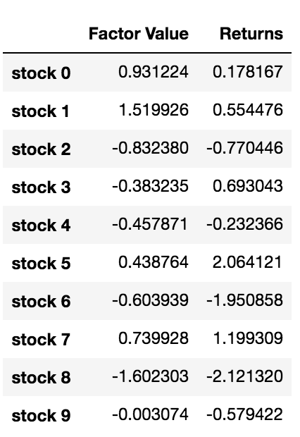
We generate and rank random indicators and random factors. Let's assume that our future returns actually depend on these factor values.

import numpy as np
import statsmodels.api as sm
import scipy.stats as stats
import scipy
import matplotlib.pyplot as plt
import seaborn as sns
import pandas as pd
## PROBLEM SETUP ##
# Generate stocks and a random factor value for them
stock_names = ['stock ' + str(x) for x in range(10000)]
current_factor_values = np.random.normal(0, 1, 10000)
# Generate future returns for these are dependent on our factor values
future_returns = current_factor_values + np.random.normal(0, 1, 10000)
# Put both the factor values and returns into one dataframe
data = pd.DataFrame(index = stock_names, columns=['Factor Value','Returns'])
data['Factor Value'] = current_factor_values
data['Returns'] = future_returns
# Take a look
data.head(10)

Now that we have the factor value and the yield, we can see what happens if we rank the benchmark based on the factor value, and then we open the overhead and the short position.

# Rank stocks
ranked_data = data.sort_values('Factor Value')
# Compute the returns of each basket with a basket size 500, so total (10000/500) baskets
number_of_baskets = int(10000/500)
basket_returns = np.zeros(number_of_baskets)
for i in range(number_of_baskets):
    start = i * 500
    end = i * 500 + 500 
    basket_returns[i] = ranked_data[start:end]['Returns'].mean()
# Plot the returns of each basket
plt.figure(figsize=(15,7))
plt.bar(range(number_of_baskets), basket_returns)
plt.ylabel('Returns')
plt.xlabel('Basket')
plt.legend(['Returns of Each Basket'])
plt.show()

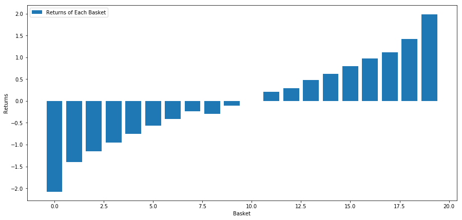
Our strategy is to get more first place in a pool of investment indicators; to get 10th place in a pool of investment indicators; the payoff of this strategy is:

basket_returns[number_of_baskets-1] - basket_returns[0]

The result is: 4.172.

Put money into our ranking model so that it can separate the high performers from the low performers.

Later in this article, we will discuss how to evaluate ranking schemes. The advantage of ranking-based arbitrage is that it is not affected by market disorder but can be exploited.

Let's consider a real-world example.

We uploaded data for 32 stocks in different sectors of the S&P 500 and tried to rank them.

from backtester.dataSource.yahoo_data_source import YahooStockDataSource
from datetime import datetime
startDateStr = '2010/01/01'
endDateStr = '2017/12/31'
cachedFolderName = '/Users/chandinijain/Auquan/yahooData/'
dataSetId = 'testLongShortTrading'
instrumentIds = ['ABT','AKS','AMGN','AMD','AXP','BK','BSX',
                'CMCSA','CVS','DIS','EA','EOG','GLW','HAL',
                'HD','LOW','KO','LLY','MCD','MET','NEM',
                'PEP','PG','M','SWN','T','TGT',
                'TWX','TXN','USB','VZ','WFC']
ds = YahooStockDataSource(cachedFolderName=cachedFolderName,
                            dataSetId=dataSetId,
                            instrumentIds=instrumentIds,
                            startDateStr=startDateStr,
                            endDateStr=endDateStr,
                            event='history')
price = 'adjClose'

Let's use a standardized momentum indicator over a monthly time period as a basis for ranking.

## Define normalized momentum
def momentum(dataDf, period):
    return dataDf.sub(dataDf.shift(period), fill_value=0) / dataDf.iloc[-1]
## Load relevant prices in a dataframe
data = ds.getBookDataByFeature()[‘Adj Close’]
#Let's load momentum score and returns into separate dataframes
index = data.index
mscores = pd.DataFrame(index=index,columns=assetList)
mscores = momentum(data, 30)
returns = pd.DataFrame(index=index,columns=assetList)
day = 30

Now we will analyze the behavior of our stock to see how our stock performs in the market in our chosen ranking factors.

Analyzing the data

The behaviour of stocks

Let's see how the stock in the basket we chose performs in our ranking model. For this, let's calculate the weekly long-term returns of all the stocks. Then we can look at the correlation of each stock's return to a week ago to the previous 30-day momentum. Stocks that show positive correlation are trend-followers, and stocks that show negative correlation are mean return.

# Calculate Forward returns
forward_return_day = 5
returns = data.shift(-forward_return_day)/data -1
returns.dropna(inplace = True)
# Calculate correlations between momentum and returns
correlations = pd.DataFrame(index = returns.columns, columns = [‘Scores’, ‘pvalues’])
mscores = mscores[mscores.index.isin(returns.index)]
for i in correlations.index:
    score, pvalue = stats.spearmanr(mscores[i], returns[i])
    correlations[‘pvalues’].loc[i] = pvalue
    correlations[‘Scores’].loc[i] = score
correlations.dropna(inplace = True)
correlations.sort_values(‘Scores’, inplace=True)
l = correlations.index.size
plt.figure(figsize=(15,7))
plt.bar(range(1,1+l),correlations[‘Scores’])
plt.xlabel(‘Stocks’)
plt.xlim((1, l+1))
plt.xticks(range(1,1+l), correlations.index)
plt.legend([‘Correlation over All Data’])
plt.ylabel(‘Correlation between %s day Momentum Scores and %s-day forward returns by Stock’%(day,forward_return_day));
plt.show()

All of our stocks have some degree of even-valued returns! (Obviously that's how the universe we chose works) This tells us that if a stock scores highly in momentum analysis, we should expect it to perform poorly next week.

Relation between scoring and earnings in dynamic analysis

Next, we need to look at the correlation between our ranking scores and the overall forward returns of the market, i.e. whether the prediction of expected returns is related to our ranking factors, and whether higher levels of correlation predict poorer relative returns, or vice versa.

To do this, we calculated the daily correlation between the 30-day momentum of all stocks and the one-week long-term return.

correl_scores = pd.DataFrame(index = returns.index.intersection(mscores.index), columns = [‘Scores’, ‘pvalues’])
for i in correl_scores.index:
    score, pvalue = stats.spearmanr(mscores.loc[i], returns.loc[i])
    correl_scores[‘pvalues’].loc[i] = pvalue
    correl_scores[‘Scores’].loc[i] = score
correl_scores.dropna(inplace = True)
l = correl_scores.index.size
plt.figure(figsize=(15,7))
plt.bar(range(1,1+l),correl_scores[‘Scores’])
plt.hlines(np.mean(correl_scores[‘Scores’]), 1,l+1, colors=’r’, linestyles=’dashed’)
plt.xlabel(‘Day’)
plt.xlim((1, l+1))
plt.legend([‘Mean Correlation over All Data’, ‘Daily Rank Correlation’])
plt.ylabel(‘Rank correlation between %s day Momentum Scores and %s-day forward returns’%(day,forward_return_day));
plt.show()

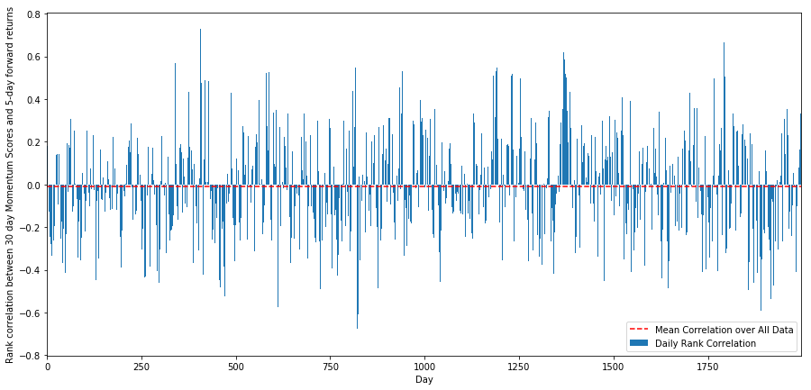
The daily correlation is very noisy, but very slight (which is to be expected, because we said all stocks will return at par value). We also look at the average monthly correlation to the return one month ago.

monthly_mean_correl =correl_scores['Scores'].astype(float).resample('M').mean()
plt.figure(figsize=(15,7))
plt.bar(range(1,len(monthly_mean_correl)+1), monthly_mean_correl)
plt.hlines(np.mean(monthly_mean_correl), 1,len(monthly_mean_correl)+1, colors='r', linestyles='dashed')
plt.xlabel('Month')
plt.xlim((1, len(monthly_mean_correl)+1))
plt.legend(['Mean Correlation over All Data', 'Monthly Rank Correlation'])
plt.ylabel('Rank correlation between %s day Momentum Scores and %s-day forward returns'%(day,forward_return_day));
plt.show()

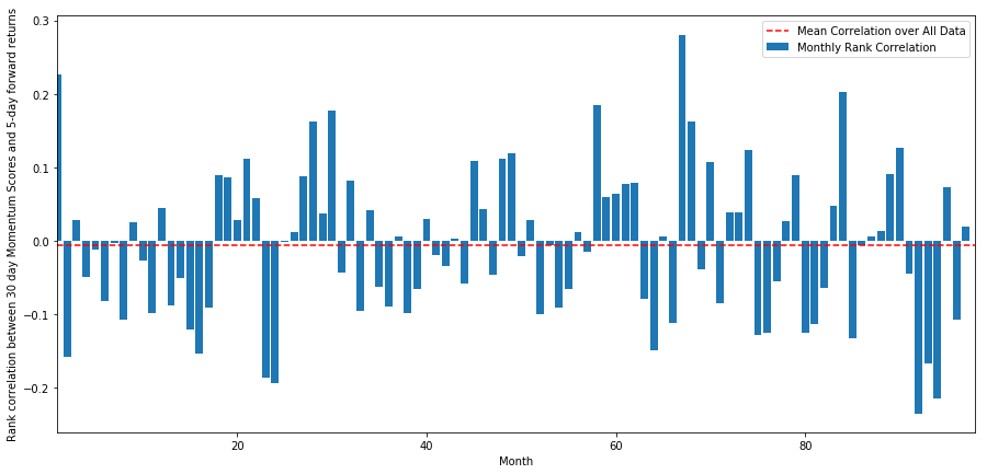
We can see that the average correlation is again slightly negative, but it also varies greatly from month to month.

Average return on a basket of stocks

We've calculated the return of a basket of stocks taken out of our ranking. If we rank all the stocks and divide them into nn groups, what is the average return of each group?

The first step is to create a function that will give the average return and ranking factors for each given basket per month.

def compute_basket_returns(factor, forward_returns, number_of_baskets, index):
data = pd.concat([factor.loc[index],forward_returns.loc[index]], axis=1)
    # Rank the equities on the factor values
    data.columns = ['Factor Value', 'Forward Returns']
    data.sort_values('Factor Value', inplace=True)
    # How many equities per basket
    equities_per_basket = np.floor(len(data.index) / number_of_baskets)
basket_returns = np.zeros(number_of_baskets)
# Compute the returns of each basket
    for i in range(number_of_baskets):
        start = i * equities_per_basket
        if i == number_of_baskets - 1:
            # Handle having a few extra in the last basket when our number of equities doesn't divide well
            end = len(data.index) - 1
        else:
            end = i * equities_per_basket + equities_per_basket
        # Actually compute the mean returns for each basket
        #s = data.index.iloc[start]
        #e = data.index.iloc[end]
        basket_returns[i] = data.iloc[int(start):int(end)]['Forward Returns'].mean()
        
    return basket_returns

When we rank stocks based on this score, we calculate the average return of each basket. This should give us an idea of their relationship over a long period of time.

number_of_baskets = 8
mean_basket_returns = np.zeros(number_of_baskets)
resampled_scores = mscores.astype(float).resample('2D').last()
resampled_prices = data.astype(float).resample('2D').last()
resampled_scores.dropna(inplace=True)
resampled_prices.dropna(inplace=True)
forward_returns = resampled_prices.shift(-1)/resampled_prices -1
forward_returns.dropna(inplace = True)
for m in forward_returns.index.intersection(resampled_scores.index):
    basket_returns = compute_basket_returns(resampled_scores, forward_returns, number_of_baskets, m)
    mean_basket_returns += basket_returns
mean_basket_returns /= l    
print(mean_basket_returns)
# Plot the returns of each basket
plt.figure(figsize=(15,7))
plt.bar(range(number_of_baskets), mean_basket_returns)
plt.ylabel('Returns')
plt.xlabel('Basket')
plt.legend(['Returns of Each Basket'])
plt.show()

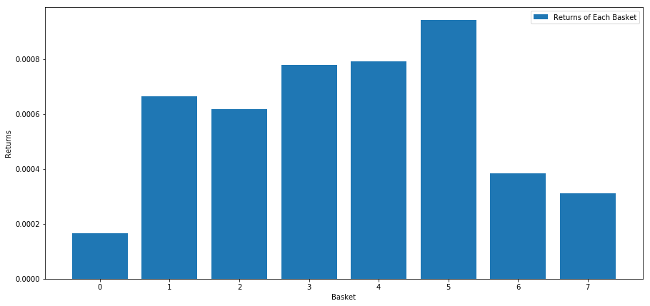
It seems that we have managed to separate the high performers from the low performers.

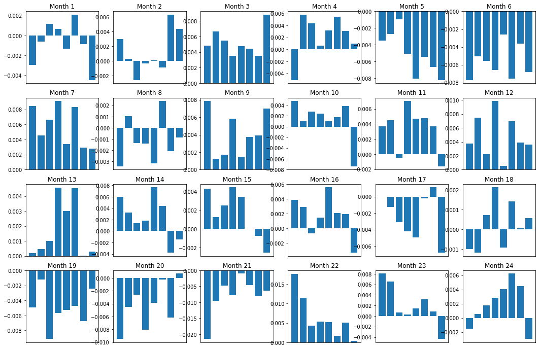
Consistency of the profit margin

Of course, these are just averages. To understand how consistent this relationship is and whether we are willing to trade, we should change the way and attitude we view it over time. Next, we'll look at the monthly interest rate differential (the "kiffer") for the first two years of them.

total_months = mscores.resample('M').last().index
months_to_plot = 24
monthly_index = total_months[:months_to_plot+1]
mean_basket_returns = np.zeros(number_of_baskets)
strategy_returns = pd.Series(index = monthly_index)
f, axarr = plt.subplots(1+int(monthly_index.size/6), 6,figsize=(18, 15))
for month in range(1, monthly_index.size):
    temp_returns = forward_returns.loc[monthly_index[month-1]:monthly_index[month]]
    temp_scores = resampled_scores.loc[monthly_index[month-1]:monthly_index[month]]
    for m in temp_returns.index.intersection(temp_scores.index):
        basket_returns = compute_basket_returns(temp_scores, temp_returns, number_of_baskets, m)
        mean_basket_returns += basket_returns
    
    strategy_returns[monthly_index[month-1]] = mean_basket_returns[ number_of_baskets-1] - mean_basket_returns[0]
    
    mean_basket_returns /= temp_returns.index.intersection(temp_scores.index).size
    
    r = int(np.floor((month-1) / 6))
    c = (month-1) % 6
    axarr[r, c].bar(range(number_of_baskets), mean_basket_returns)
    axarr[r, c].xaxis.set_visible(False)
    axarr[r, c].set_title('Month ' + str(month))
plt.show()

plt.figure(figsize=(15,7))
plt.plot(strategy_returns)
plt.ylabel(‘Returns’)
plt.xlabel(‘Month’)
plt.plot(strategy_returns.cumsum())
plt.legend([‘Monthly Strategy Returns’,’Cumulative Strategy Returns’])
plt.show()

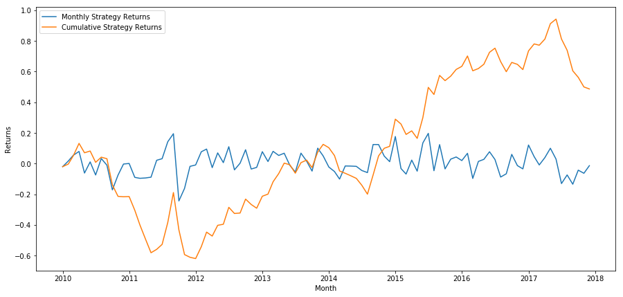
Finally, if we do the last basket and empty the first basket every month, then let's look at the return (assuming the equity distribution of each security)

total_return = strategy_returns.sum()
ann_return = 100*((1 + total_return)**(12.0 /float(strategy_returns.index.size))-1)
print('Annual Returns: %.2f%%'%ann_return)

Annual rate of return: 5.03%

We see that we have a very weak ranking scheme that only modestly differentiates high-performing stocks from low-performing stocks.

Finding the Right Ranking

In order to implement a multi-space balancing strategy, you actually just need to define a ranking scheme. Everything else is mechanical. Once you have a multi-space balancing strategy, you can swap different ranking factors, and nothing else requires too many changes. This is a very convenient way to quickly iterate your ideas without worrying about adjusting all the code every time.

Ranking schemes can also come from almost any model. It is not necessarily a value-based factor model, it can be a machine learning technique that predicts returns a month in advance and ranks based on that ranking.

Selection and evaluation of ranking schemes

Ranking schemes are the strengths and the most important component of a multi-space balancing strategy. Choosing a good ranking scheme is a systematic process, and there are no easy answers.

A good place to start is to pick existing known technologies and see if you can modify them slightly for higher returns.

• Cloning and adjustmentChoose a topic that is frequently discussed and see if you can modify it slightly to gain an advantage. In most cases, public factors will no longer have trading signals because they are fully capitalized out of the market. However, sometimes they will guide you in the right direction.

• Pricing model: Any model that predicts future returns can be a factor and has the potential to be used to rank your basket of trading indicators. You can take any complex pricing model and convert it to a ranking scheme.

• Factors based on price (technical indicators)Price-based factors, as we discussed today, get information about the historical price of each interest and use it to generate factor values. Examples might be moving averages, momentum indicators, or volatility indicators.

• Regression and momentumIt is noteworthy that some factors assume that prices will continue to move in one direction once they do; some factors are just the opposite. Both are valid models of different time scales and assets, and it is important to study whether underlying behavior is based on momentum or on regression.

• Basic factors (based on value)This is a combination of using underlying values such as PE, dividends, etc. Underlying values contain information that is relevant to the real-world facts of the company and can therefore be stronger than price in many respects.

In the end, growth predictors are an arms race, and you're trying to stay ahead of the game. Factors will be priced out of the market and have a lifespan, so you have to work constantly to determine how much your factors have declined and what new factors can be used to replace them.

Other considerations

• Re-balancing the frequency

Each ranking system will predict returns over slightly different time frames. Price-based mean value returns may be predictable in a few days, while value-based factor models may be predictive in a few months. Determining the time frame the model should predict is very important, and statistical verification is done before executing the strategy. You certainly don't want to overfit by trying to optimize the frequency of rebalancing, and you will inevitably find a random one that is optimal over other frequencies.

• Capital capacity and transaction costs

Each strategy has a minimum and maximum capital volume, and the minimum threshold is usually determined by the transaction cost.

Trading too many shares will result in high trading costs. Suppose you want to buy 1000 shares, then each rebalancing will result in several thousand dollars in costs. Your capital base must be high enough that the trading costs account for a small fraction of the returns generated by your strategy. For example, if your capital is $100,000 and your strategy earns 1% per month (($1,000), all of these returns will be taken up by the trading costs.

The lowest asset threshold depends mainly on the number of shares traded. However, the maximum capacity is also very high, and the multi-empty balancing equity strategy is able to trade hundreds of millions of dollars without losing an advantage. This is true because the strategy is relatively infrequent in rebalancing. The total assets will be very low in addition to the number of shares traded, and the dollar value of each share will be so low that you do not have to worry about your volume affecting the market.

Related

More