Implementar una estrategia de negociación cuantitativa de moneda digital de doble impulso en Python
El autor:- ¿ Por qué?, Creado: 2023-01-10 17:07:49, Actualizado: 2023-09-20 10:53:48
Implementar una estrategia de negociación cuantitativa de moneda digital de doble impulso en Python
Introducción al algoritmo de negociación de doble empuje
El algoritmo de negociación de doble empuje es una famosa estrategia de negociación cuantitativa desarrollada por Michael Chalek. Se usa generalmente en futuros, divisas y mercados de valores. El concepto de doble empuje es un sistema comercial de avance típico. Utiliza el sistema de
En este artículo, damos los detalles lógicos detallados de esta estrategia y mostramos cómo implementar este algoritmo en la plataforma FMZ Quant. En primer lugar, necesitamos seleccionar el precio histórico del tema a negociar. Este rango se calcula en función del precio de cierre, el precio más alto y el precio más bajo de los últimos N días. Cuando el mercado se mueve un cierto rango desde el precio de apertura, abra la posición.
Probamos esta estrategia con un solo par de operaciones bajo dos condiciones comunes de mercado, a saber, mercado de tendencia y mercado de choque. Los resultados mostraron que el sistema de negociación de impulso funciona mejor en el mercado de tendencia y desencadenará algunas señales comerciales inválidas en el mercado volátil. En el mercado de intervalos, podemos ajustar los parámetros para obtener mejores rendimientos. Como comparación de objetivos de negociación de referencia individuales, también probamos el mercado de futuros de productos básicos domésticos. El resultado mostró que la estrategia es mejor que el rendimiento promedio.
Principio de la estrategia de la DT
Su prototipo lógico es una estrategia comercial intradiaria común. La estrategia de avance de rango de apertura se basa en el precio de apertura de hoy más o menos un cierto porcentaje del rango de ayer para determinar las pistas superior y inferior. Cuando el precio cruza la pista superior, abrirá su posición para comprar, y cuando rompe la pista inferior, abrirá su posición para ser corto.
Principio de la estrategia
-
Después del cierre, se calculan dos valores: el precio más alto, el precio de cierre, y el precio de cierre, el precio más bajo. Luego, toma el mayor de los dos valores y multiplica el valor por 0.7.
-
Después de que el mercado se abra al día siguiente, registre el precio de apertura y compre inmediatamente cuando el precio exceda (precio de apertura + valor de activación), o venda posiciones cortas cuando el precio sea inferior a (precio de apertura - valor de activación).
-
Esta estrategia no tiene un stop loss obvio. Este sistema es un sistema inverso, es decir, si hay una orden de posición corta cuando el precio excede (precio de apertura + valor de activación), enviará dos órdenes de compra (una cierra la posición incorrecta, la otra abre la posición correcta). Por la misma razón, si el precio de una posición larga es menor que (precio de apertura - valor de activación), enviará dos órdenes de venta.
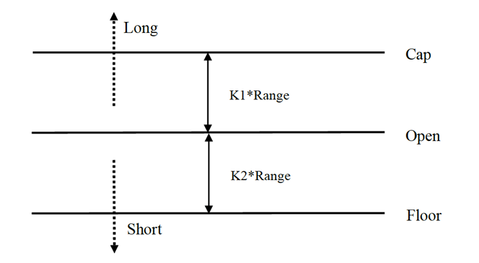
Expresión matemática de la estrategia DT
El valor de las emisiones de gases de efecto invernadero se calculará en función de las emisiones de gases de efecto invernadero de las emisiones de gases de efecto invernadero.
El método de cálculo de la señal de posición larga es el siguiente:
Cap = abierto + K1 × Rangecap = abierto + K1 × Range
El método de cálculo de la señal de posición corta es el siguiente:
el piso = abierto
Cuando K1 y K2 son parámetros. Cuando K1 es mayor que K2, se activa la señal de posición larga, y viceversa. Para la demostración, elegimos K1=K2=0.5. En las transacciones reales, todavía podemos usar datos históricos para optimizar estos parámetros o ajustar los parámetros de acuerdo con las tendencias del mercado. Si eres alcista, K1 debe ser menor que K2. Si eres bajista, K1 debe ser mayor que K2.
El sistema es un sistema de reversión. Por lo tanto, si los inversores mantienen posiciones cortas cuando el precio cruza la pista superior, deben cerrar las posiciones cortas antes de abrir posiciones largas. Si un inversor mantiene una posición larga cuando el precio rompe la pista inferior, deben cerrar la posición larga antes de abrir una nueva posición corta.
Mejora de la estrategia de la TD:
En la configuración del intervalo, se introducen los cuatro puntos de precios (alto, abierto, bajo y cerrado) de los N días anteriores para que el intervalo sea relativamente estable en un determinado período, lo que puede aplicarse al seguimiento de la tendencia diaria.
Las condiciones de activación de la apertura de posiciones largas y cortas de la estrategia, teniendo en cuenta el rango asimétrico, el rango de referencia de las transacciones largas y cortas debe seleccionar un número diferente de períodos, que también pueden determinarse por los parámetros K1 y K2.
Por lo tanto, al utilizar esta estrategia, por un lado, puede referirse a los mejores parámetros de backtesting de datos históricos. Por otro lado, puede ajustar K1 y K2 en etapas de acuerdo con su juicio del futuro u otros indicadores técnicos de período importante.
Este es un método comercial típico de esperar señales, entrar en el mercado, el arbitraje, y luego salir del mercado, pero el efecto es excelente.
Implementar la estrategia de DT en la plataforma FMZ Quant
Estamos abiertos.FMZ.COM, inicie sesión en la cuenta, haga clic en el panel de control, y desplegar el docker y el robot.
Por favor, consulte mi artículo anterior sobre cómo desplegar un docker y robot:https://www.fmz.com/bbs-topic/9864.
Los lectores que quieran comprar su propio servidor de computación en la nube para implementar dockers pueden consultar este artículo:https://www.fmz.com/digest-topic/5711.
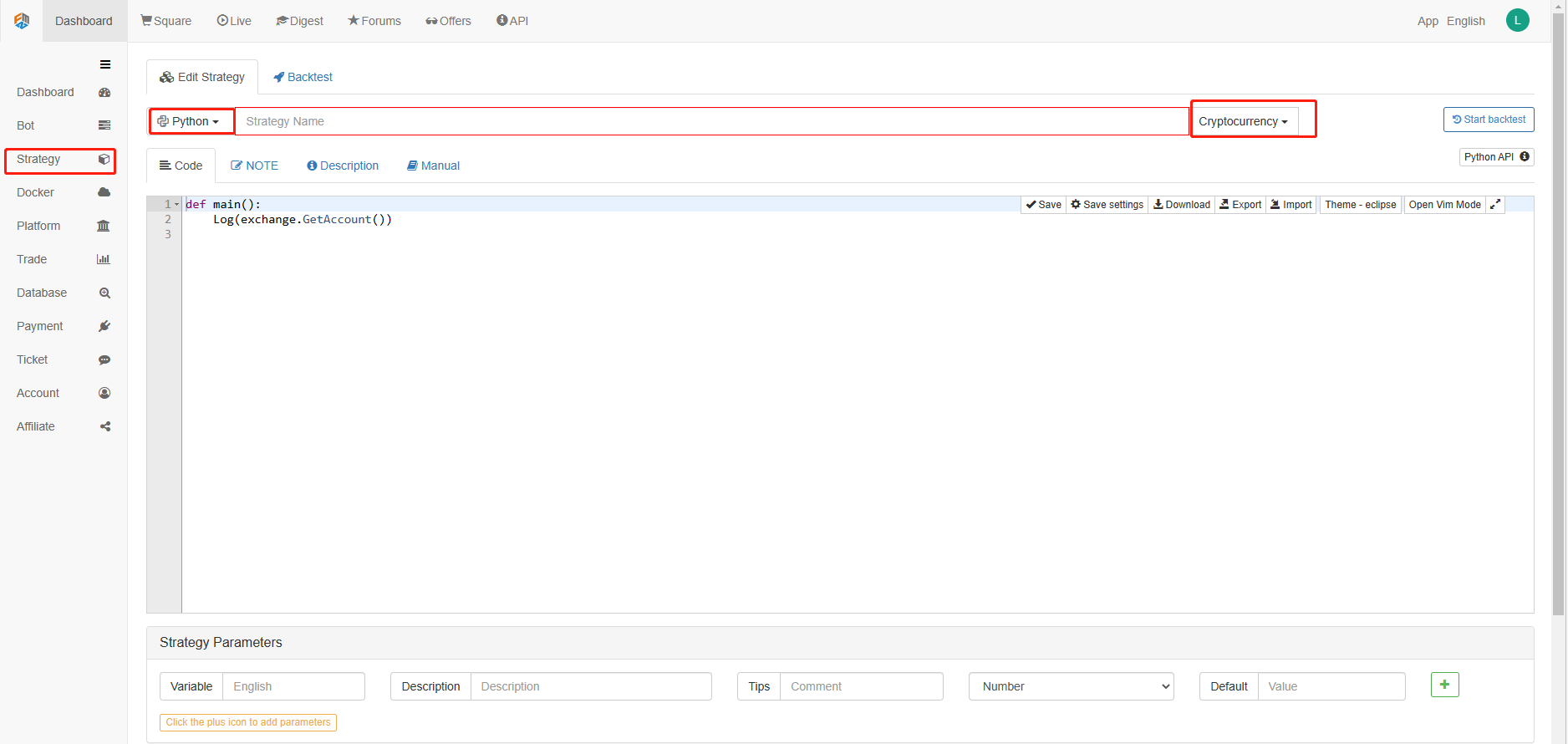
A continuación, hacemos clic en la Biblioteca de Estrategias en la columna izquierda y hacemos clic en Agregar estrategia.
Recuerde seleccionar el lenguaje de programación como Python en la esquina superior derecha de la página de edición de estrategias, como se muestra en la figura:
A continuación, escribiremos código Python en la página de edición de código. El siguiente código tiene comentarios muy detallados línea por línea, puede tomarse su tiempo para entender.
Usaremos los futuros de OKCoin para probar la estrategia:
import time # Here we need to introduce the time library that comes with python, which will be used later in the program.

class Error_noSupport(BaseException): # We define a global class named ChartCfg to initialize the strategy chart settings. Object has many attributes about the chart function. Chart library: HighCharts.
    def __init__(self): # log out prompt messages
        Log("Support OKCoin Futures only! #FF0000")

class Error_AtBeginHasPosition(BaseException):
    def __init__(self):
        Log("Start with a futures position! #FF0000")

ChartCfg = {
    '__isStock': True, # This attribute is used to control whether to display a single control data series (you can cancel the display of a single data series on the chart). If you specify __isStock: false, it will be displayed as a normal chart.
    'title': { # title is the main title of the chart
        'text': 'Dual Thrust upper and bottom track chart' # An attribute of the title text is the text of the title, here set to 'Dual Thrust upper and bottom track chart' the text will be displayed in the title position.
    },
    'yAxis': { # Settings related to the Y-axis of the chart coordinate.
        'plotLines': [{ # Horizontal lines on the Y-axis (perpendicular to the Y-axis), the value of this attribute is an array, i.e. the setting of multiple horizontal lines.
            'value': 0, # Coordinate value of horizontal line on Y-axis
            'color': 'red', # Color of horizontal line
            'width': 2, # Line width of horizontal line
            'label': {  # Labels on the horizontal line
                'text': 'Upper track', # Text of the label
                'align': 'center' # The display position of the label, here set to center (i.e.: 'center')
            },
        }, {       # The second horizontal line ([{...} , {...}] the second element in the array)
            'value': 0, # Coordinate value of horizontal line on Y-axis
            'color': 'green', # Color of horizontal line
            'width': 2,  # Line width of horizontal line
            'label': { # Label
                'text': 'bottom track',
                'align': 'center'
            },
        }]
    },
    'series': [{ # Data series, that is, data used to display data lines, K-lines, tags, and other contents on the chart. It is also an array whose first index is 0.
        'type': 'candlestick', # Type of data series with index 0: 'candlestick' indicates a K-line chart.
        'name': 'Current period',  # Name of the data series
        'id': 'primary', # The ID of the data series, which is used for the related settings of the next data series.
        'data': []  # An array of data series to store specific K-line data
    }, {
        'type': 'flags',  # Data series, type: 'flags', display labels on the chart, indicating going long and going short. Index is 1.
        'onSeries': 'primary',  # This attribute indicates that the label is displayed on id 'primary'.
        'data': []    # The array that holds the label data.
    }]
}

STATE_IDLE = 0  # Status constants, indicating idle
STATE_LONG = 1 # Status constants, indicating long positions
STATE_SHORT = 2 # Status constants, indicating short positions
State = STATE_IDLE # Indicates the current program status, assigned as idle initially

LastBarTime = 0  # The time stamp of the last column of the K-line (in milliseconds, 1000 milliseconds is equal to 1 second, and the timestamp is the number of milliseconds from January 1, 1970 to the present time is a large positive integer).
UpTrack = 0   # Upper track value
BottomTrack = 0 # Bottom track value
chart = None # It is used to accept the chart control object returned by the Chart API function. Use this object (chart) to call its member function to write data to the chart.
InitAccount = None # Initial account status
LastAccount = None # Latest account status
Counter = { # Counters for recording profit and loss counts
    'w': 0, # Number of wins
    'l': 0  # Number of losses
}

def GetPosition(posType):  # Define a function to store account position information
    positions = exchange.GetPosition() # exchange.GetPosition() is the FMZ Quant official API. For its usage, please refer to the official API document: https://www.fmz.com/api.
    return [{'Price': position['Price'], 'Amount': position['Amount']} for position in positions if position['Type'] == posType] # Return to various position information

def CancelPendingOrders(): # Define a function specifically for withdrawing orders
    while True: # Loop check
        orders = exchange.GetOrders() # If there is a position
        [exchange.CancelOrder(order['Id']) for order in orders if not Sleep(500)] # Withdrawal statement
        if len(orders) == 0: # Logical judgment
            break

def Trade(currentState,nextState): # Define a function to determine the order placement logic.
    global InitAccount,LastAccount,OpenPrice,ClosePrice # Define the global scope
    ticker = _C(exchange.GetTicker) # For the usage of _C, please refer to: https://www.fmz.com/api.
    slidePrice = 1 # Define the slippage value
    pfn = exchange.Buy if nextState == STATE_LONG else exchange.Sell # Buying and selling judgment logic
    if currentState != STATE_IDLE: # Loop start
        Log(_C(exchange.GetPosition)) # Log information
        exchange.SetDirection("closebuy" if currentState == STATE_LONG else "closesell") # Adjust the order direction, especially after placing the order.
        while True:
            ID = pfn( (ticker['Last'] - slidePrice) if currentState == STATE_LONG else (ticker['Last'] + slidePrice), AmountOP) # Price limit order, ID=pfn (- 1, AmountOP) is the market price order, ID=pfn (AmountOP) is the market price order.
            Sleep(Interval) # Take a break to prevent the API from being accessed too often and your account being blocked.
            Log(exchange.GetOrder(ID)) # Log information
            ClosePrice = (exchange.GetOrder(ID))['AvgPrice'] # Set the closing price
            CancelPendingOrders() # Call the withdrawal function
            if len(GetPosition(PD_LONG if currentState == STATE_LONG else PD_SHORT)) == 0: # Order withdrawal logic
                break
        account = exchange.GetAccount() # Get account information
        if account['Stocks'] > LastAccount['Stocks']: # If the current account currency value is greater than the previous account currency value.
            Counter['w'] += 1 # In the profit and loss counter, add one to the number of profits.
        else:
            Counter['l'] += 1 # Otherwise, add one to the number of losses.
        Log(account) # log information
        LogProfit((account['Stocks'] - InitAccount['Stocks']),"Return rates:", ((account['Stocks'] - InitAccount['Stocks']) * 100 / InitAccount['Stocks']),'%')
        Cal(OpenPrice,ClosePrice)
        LastAccount = account

    exchange.SetDirection("buy" if nextState == STATE_LONG else "sell") # The logic of this part is the same as above and will not be elaborated.
    Log(_C(exchange.GetAccount))
    while True:
        ID = pfn( (ticker['Last'] + slidePrice) if nextState == STATE_LONG else (ticker['Last'] - slidePrice), AmountOP)
        Sleep(Interval)
        Log(exchange.GetOrder(ID))
        CancelPendingOrders()
        pos = GetPosition(PD_LONG if nextState == STATE_LONG else PD_SHORT)
        if len(pos) != 0:
            Log("Average price of positions",pos[0]['Price'],"Amount:",pos[0]['Amount'])
            OpenPrice = (exchange.GetOrder(ID))['AvgPrice']
            Log("now account:",exchange.GetAccount())
            break

def onTick(exchange): # The main function of the program, within which the main logic of the program is processed.
    global LastBarTime,chart,State,UpTrack,DownTrack,LastAccount # Define the global scope
    records = exchange.GetRecords() # For the usage of exchange.GetRecords(), please refer to: https://www.fmz.com/api.
    if not records or len(records) <= NPeriod: # Judgment statements to prevent accidents.
        return
    Bar = records[-1] # Take the penultimate element of records K-line data, that is, the last bar.
    if LastBarTime != Bar['Time']:
        HH = TA.Highest(records, NPeriod, 'High')  # Declare the HH variable, call the TA.Highest function to calculate the maximum value of the highest price in the current K-line data NPeriod period and assign it to HH.
        HC = TA.Highest(records, NPeriod, 'Close') # Declare the HC variable to get the maximum value of the closing price in the NPeriod period.
        LL = TA.Lowest(records, NPeriod, 'Low') # Declare the LL variable to get the minimum value of the lowest price in the NPeriod period.
        LC = TA.Lowest(records, NPeriod, 'Close') # Declare LC variable to get the minimum value of the closing price in the NPeriod period. For specific TA-related applications, please refer to the official API documentation.

        Range = max(HH - LC, HC - LL)  # Calculate the range
        UpTrack = _N(Bar['Open'] + (Ks * Range))  # The upper track value is calculated based on the upper track factor Ks of the interface parameters such as the opening price of the latest K-line bar.
        DownTrack = _N(Bar['Open'] - (Kx * Range)) # Calculate the down track value
        if LastBarTime > 0: # Because the value of LastBarTime initialization is set to 0, LastBarTime>0 must be false when running here for the first time. The code in the if block will not be executed, but the code in the else block will be executed.
            PreBar = records[-2] # Declare a variable means "the previous Bar" assigns the value of the penultimate Bar of the current K-line to it.
            chart.add(0, [PreBar['Time'], PreBar['Open'], PreBar['High'], PreBar['Low'], PreBar['Close']], -1) # Call the add function of the chart icon control class to update the K-line data (use the penultimate bar of the obtained K-line data to update the last bar of the icon, because a new K-line bar is generated).
        else:  # For the specific usage of the chart.add function, see the API documentation and the articles in the forum. When the program runs for the first time, it must execute the code in the else block. The main function is to add all the K-lines obtained for the first time to the chart at one time.
            for i in range(len(records) - min(len(records), NPeriod * 3), len(records)): # Here, a for loop is executed. The number of loops uses the minimum of the K-line length and 3 times the NPeriod, which can ensure that the initial K-line will not be drawn too much and too long. Indexes vary from large to small.
                b = records[i] # Declare a temporary variable b to retrieve the K-line bar data with the index of records.length - i for each loop.
                chart.add(0,[b['Time'], b['Open'], b['High'], b['Low'], b['Close']]) # Call the chart.add function to add a K-line bar to the chart. Note that if the last parameter of the add function is passed in -1, it will update the last Bar (column) on the chart. If no parameter is passed in, it will add Bar to the last. After executing the loop of i=2 (i-- already, now it's 1), it will trigger i > 1 for false to stop the loop. It can be seen that the code here only processes the bar of records.length - 2, and the last Bar is not processed.
        chart.add(0,[Bar['Time'], Bar['Open'], Bar['High'], Bar['Low'], Bar['Close']]) # Since the two branches of the above if do not process the bar of records.length - 1, it is processed here. Add the latest Bar to the chart.
        ChartCfg['yAxis']['plotLines'][0]['value'] = UpTrack  # Assign the calculated upper track value to the chart object (different from the chart control object chart) for later display.
        ChartCfg['yAxis']['plotLines'][1]['value'] = DownTrack # Assign lower track value
        ChartCfg['subtitle'] = { # Set subtitle
            'text': 'upper tarck' + str(UpTrack) + 'down track' + str(DownTrack) # Subtitle text setting. The upper and down track values are displayed on the subtitle.
        }
        chart.update(ChartCfg) # Update charts with chart class ChartCfg.
        chart.reset(PeriodShow) # Refresh the PeriodShow variable set according to the interface parameters, and only keep the K-line bar of the number of PeriodShow values.

        LastBarTime = Bar['Time'] # The timestamp of the newly generated Bar is updated to LastBarTime to determine whether the last Bar of the K-line data acquired in the next loop is a newly generated one.
    else: # If LastBarTime is equal to Bar.Time, that is, no new K-line Bar is generated. Then execute the code in {..}.
        chart.add(0,[Bar['Time'], Bar['Open'], Bar['High'], Bar['Low'], Bar['Close']], -1) # Update the last K-line bar on the chart with the last Bar of the current K-line data (the last Bar of the K-line, i.e. the Bar of the current period, is constantly changing).
    LogStatus("Price:", Bar["Close"], "up:", UpTrack, "down:", DownTrack, "wins:", Counter['w'], "losses:", Counter['l'], "Date:", time.time()) # The LogStatus function is called to display the data of the current strategy on the status bar.
    msg = "" # Define a variable msg.
    if State == STATE_IDLE or State == STATE_SHORT: # Judge whether the current state variable State is equal to idle or whether State is equal to short position. In the idle state, it can trigger long position, and in the short position state, it can trigger a long position to be closed and sell the opening position.
        if Bar['Close'] >= UpTrack: # If the closing price of the current K-line is greater than the upper track value, execute the code in the if block.
            msg = "Go long, trigger price:" + str(Bar['Close']) + "upper track" + str(UpTrack) # Assign a value to msg and combine the values to be displayed into a string.
            Log(msg) # message
            Trade(State, STATE_LONG) # Call the Trade function above to trade.
            State = STATE_LONG # Regardless of opening long positions or selling the opening position, the program status should be updated to hold long positions at the moment.
            chart.add(1,{'x': Bar['Time'], 'color': 'red', 'shape': 'flag', 'title': 'long', 'text': msg}) # Add a marker to the corresponding position of the K-line to show the open long position.

    if State == STATE_IDLE or State == STATE_LONG: # The short direction is the same as the above, and will not be repeated. The code is exactly the same.
        if Bar['Close'] <= DownTrack:
            msg = "Go short, trigger price:" + str(Bar['Close']) + "down track" + str(DownTrack)
            Log(msg)
            Trade(State, STATE_SHORT)
            State = STATE_SHORT
            chart.add(1,{'x': Bar['Time'], 'color': 'green', 'shape': 'circlepin', 'title': 'short', 'text': msg})

OpenPrice = 0 # Initialize OpenPrice and ClosePrice
ClosePrice = 0
def Cal(OpenPrice, ClosePrice): # Define a Cal function to calculate the profit and loss of the strategy after it has been run.
    global AmountOP,State
    if State == STATE_SHORT:
        Log(AmountOP,OpenPrice,ClosePrice,"Profit and loss of the strategy:", (AmountOP * 100) / ClosePrice - (AmountOP * 100) / OpenPrice, "Currencies, service charge:", - (100 * AmountOP * 0.0003), "USD, equivalent to:", _N( - 100 * AmountOP * 0.0003/OpenPrice,8), "Currencies")
        Log(((AmountOP * 100) / ClosePrice - (AmountOP * 100) / OpenPrice) + (- 100 * AmountOP * 0.0003/OpenPrice))
    if State == STATE_LONG:
        Log(AmountOP,OpenPrice,ClosePrice,"Profit and loss of the strategy:", (AmountOP * 100) / OpenPrice - (AmountOP * 100) / ClosePrice, "Currencies, service charge:", - (100 * AmountOP * 0.0003), "USD, equivalent to:", _N( - 100 * AmountOP * 0.0003/OpenPrice,8), "Currencies")
        Log(((AmountOP * 100) / OpenPrice - (AmountOP * 100) / ClosePrice) + (- 100 * AmountOP * 0.0003/OpenPrice))

def main(): # The main function of the strategy program. (entry function)
    global LoopInterval,chart,LastAccount,InitAccount # Define the global scope
    if exchange.GetName() != 'Futures_OKCoin':  # Judge if the name of the added exchange object (obtained by the exchange.GetName function) is not equal to 'Futures_OKCoin', that is, the object added is not OKCoin futures exchange object.
        raise Error_noSupport # Throw an exception
    exchange.SetRate(1) # Set various parameters of the exchange.
    exchange.SetContractType(["this_week","next_week","quarter"][ContractTypeIdx])  # Determine which specific contract to trade.
    exchange.SetMarginLevel([10,20][MarginLevelIdx]) # Set the margin rate, also known as leverage.

    if len(exchange.GetPosition()) > 0: # Set up fault tolerance mechanism.
        raise Error_AtBeginHasPosition
    CancelPendingOrders()
    InitAccount = LastAccount = exchange.GetAccount()
    LoopInterval = min(1,LoopInterval)
    Log("Trading platforms:",exchange.GetName(), InitAccount)
    LogStatus("Ready...")

    LogProfitReset()
    chart = Chart(ChartCfg)
    chart.reset()

    LoopInterval = max(LoopInterval, 1)
    while True: # Loop the whole transaction logic and call the onTick function.
        onTick(exchange)
        Sleep(LoopInterval * 1000) # Take a break to prevent the API from being accessed too frequently and the account from being blocked.
Después de escribir el código, tenga en cuenta que no hemos terminado toda la estrategia. A continuación, debemos agregar los parámetros utilizados en la estrategia a la página de edición de estrategia. El método de adición es muy simple. Simplemente haga clic en el signo más en la parte inferior del cuadro de diálogo de escritura de estrategia para agregar uno por uno.
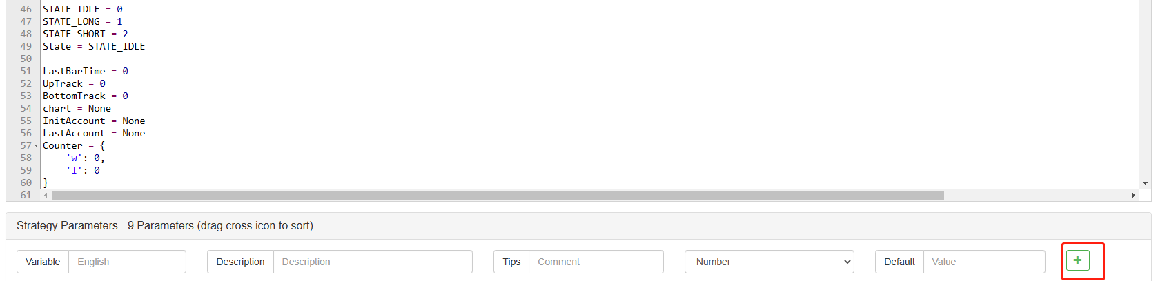
Contenido a añadir:
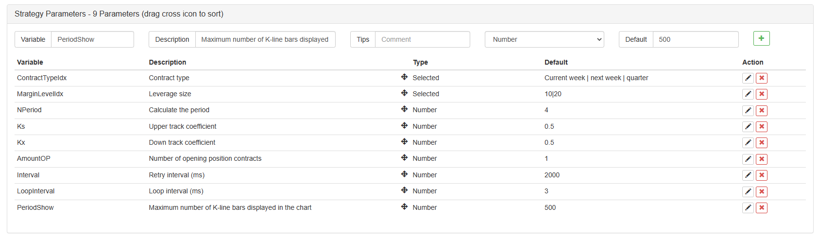
Hasta ahora, finalmente hemos completado la redacción de la estrategia.
Prueba posterior de la estrategia
Después de escribir la estrategia, lo primero que debemos hacer es hacer una prueba de retroceso para ver cómo se comporta en los datos históricos. Pero tenga en cuenta que el resultado de la prueba de retroceso no es igual a la predicción del futuro. La prueba de retroceso solo puede usarse como referencia para considerar la efectividad de nuestra estrategia. Una vez que el mercado cambia y la estrategia comienza a tener grandes pérdidas, debemos encontrar el problema a tiempo, y luego cambiar la estrategia para adaptarnos al nuevo entorno del mercado, como el umbral mencionado anteriormente. Si la estrategia tiene una pérdida mayor al 10%, debemos detener inmediatamente la operación de la estrategia, y luego encontrar el problema. Podemos comenzar a ajustar el umbral.
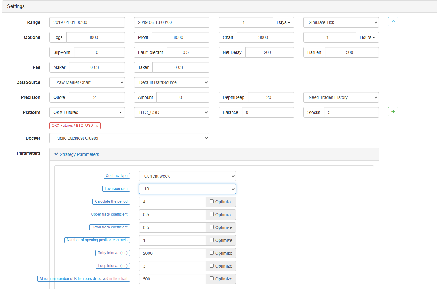
Haga clic en backtest en la página de edición de la estrategia. En la página de backtest, el ajuste de parámetros se puede llevar a cabo de manera conveniente y rápida de acuerdo con diferentes necesidades. Especialmente para la estrategia con lógica compleja y muchos parámetros, no es necesario volver al código fuente y modificarlo uno por uno.
El tiempo de prueba de retroceso es los últimos seis meses. Haga clic en Agregar el intercambio de futuros OKCoin y seleccione el objetivo de negociación de BTC.
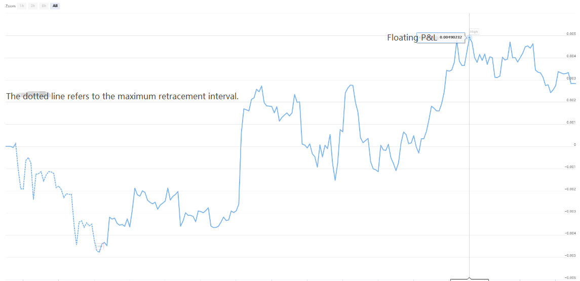
Se puede ver que la estrategia ha cosechado buenos rendimientos en los últimos seis meses debido a la muy buena tendencia unilateral de BTC.

Si tiene alguna pregunta, puede dejar un mensaje enhttps://www.fmz.com/bbs, ya se trate de la estrategia o la tecnología de la plataforma, la plataforma FMZ Quant tiene profesionales listos para responder a sus preguntas.
- Cuantificar el análisis fundamental en el mercado de criptomonedas: ¡Deja que los datos hablen por sí mismos!
- La investigación cuantitativa básica del círculo monetario - ¡No confíes más en los profesores de idiomas, los datos hablan objetivamente!
- Una herramienta esencial en el campo de la transacción cuantitativa - inventor de módulos de exploración de datos cuantitativos
- Dominarlo todo - Introducción a FMZ Nueva versión de la terminal de negociación (con el código fuente de TRB Arbitrage)
- Conozca todo acerca de la nueva versión del terminal de operaciones de FMZ (con código de código de TRB)
- FMZ Quant: Análisis de ejemplos de diseño de requisitos comunes en el mercado de criptomonedas (II)
- Cómo explotar robots de venta sin cerebro con una estrategia de alta frecuencia en 80 líneas de código
- Cuantificación FMZ: Desarrollo de casos de diseño de necesidades comunes en el mercado de criptomonedas (II)
- Cómo utilizar una estrategia de alta frecuencia de 80 líneas de código para explotar y vender robots sin cerebro
- FMZ Quant: Análisis de ejemplos de diseño de requisitos comunes en el mercado de criptomonedas (I)
- Cuantificación FMZ: Desarrollo de casos de diseño de necesidades comunes en el mercado de criptomonedas (1)