Mettre en œuvre une stratégie de négociation quantitative de monnaie numérique à double poussée en Python
Auteur:Je ne sais pas., Créé: 2023-01-10 17:07:49, Mis à jour: 2023-09-20 10:53:48
Mettre en œuvre une stratégie de négociation quantitative de monnaie numérique à double poussée en Python
Introduction à l'algorithme de négociation à double poussée
L'algorithme de trading à double poussée est une célèbre stratégie de trading quantitative développée par Michael Chalek. Il est généralement utilisé sur les marchés à terme, de change et boursiers. Le concept de double poussée est un système de trading de percée typique. Il utilise le système de
Dans cet article, nous donnons les détails logiques détaillés de cette stratégie et montrons comment mettre en œuvre cet algorithme sur la plateforme FMZ Quant. Tout d'abord, nous devons sélectionner le prix historique de l'objet à négocier. Cette plage est calculée en fonction du prix de clôture, du prix le plus élevé et du prix le plus bas des derniers jours N. Lorsque le marché se déplace dans une certaine plage par rapport au prix d'ouverture, ouvrez la position.
Nous avons testé cette stratégie avec une seule paire de négociation dans deux conditions de marché communes, à savoir le marché de tendance et le marché de choc. Les résultats ont montré que le système de négociation de l'élan fonctionne mieux sur le marché de tendance et qu'il déclenchera certains signaux de négociation invalides sur le marché volatil. Sur le marché d'intervalle, nous pouvons ajuster les paramètres pour obtenir de meilleurs rendements. Pour comparer les objectifs de négociation de référence individuels, nous avons également testé le marché intérieur des contrats à terme sur matières premières. Le résultat a montré que la stratégie est meilleure que la performance moyenne.
Principe stratégique de la DT
Son prototype logique est une stratégie de trading intraday commune. La stratégie de rupture de gamme d'ouverture est basée sur le prix d'ouverture d'aujourd'hui plus ou moins un certain pourcentage de la gamme d'hier pour déterminer les pistes supérieures et inférieures. Lorsque le prix traverse la piste supérieure, il ouvrira sa position pour acheter, et lorsqu'il brise la piste inférieure, il ouvrira sa position pour être court.
Principe de stratégie
-
Après la clôture, deux valeurs sont calculées: le prix le plus élevé - le prix de clôture, et le prix de clôture - le prix le plus bas. Ensuite, prenez le plus grand des deux valeurs et multipliez la valeur par 0,7.
-
Après l'ouverture du marché le lendemain, enregistrez le prix d'ouverture et achetez immédiatement lorsque le prix est supérieur (prix d'ouverture + valeur de déclenchement) ou vendez des positions courtes lorsque le prix est inférieur à (prix d'ouverture - valeur de déclenchement).
-
Cette stratégie n'a pas de stop loss évident. Ce système est un système inverse, c'est-à-dire que s'il y a un ordre de position courte lorsque le prix dépasse (prix d'ouverture + valeur de déclenchement), il enverra deux ordres d'achat (l'un ferme la mauvaise position, l'autre ouvre la bonne position). Pour la même raison, si le prix d'une position longue est inférieur à (prix d'ouverture - valeur de déclenchement), il enverra deux ordres de vente.
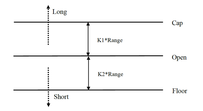
Expression mathématique de la stratégie TD
L'échantillon doit être présenté à l'échantillon.
La méthode de calcul du signal de position longue est:
Cap = ouvert + K1 × Rangecap = ouvert + K1 × Range
La méthode de calcul du signal de position courte est:
plancher = ouvert
Lorsque K1 et K2 sont des paramètres. Lorsque K1 est supérieur à K2, le signal de position longue est déclenché, et vice versa. Pour la démonstration, nous choisissons K1=K2=0.5. Dans les transactions réelles, nous pouvons toujours utiliser les données historiques pour optimiser ces paramètres ou ajuster les paramètres en fonction des tendances du marché. Si vous êtes haussier, K1 devrait être inférieur à K2. Si vous êtes baissier, K1 devrait être supérieur à K2.
Le système est un système d'inversion. Par conséquent, si les investisseurs détiennent des positions courtes lorsque le prix franchit la voie supérieure, ils devraient fermer les positions courtes avant d'ouvrir des positions longues. Si un investisseur détient une position longue lorsque le prix franchit la voie inférieure, il devrait fermer la position longue avant d'ouvrir une nouvelle position courte.
Amélioration de la stratégie de la TD:
Dans le paramètre d'intervalle, les quatre points de prix (haute, ouverte, basse et fermée) des N jours précédents sont introduits pour rendre l'intervalle relativement stable sur une certaine période, ce qui peut être appliqué au suivi de la tendance quotidienne.
Les conditions de déclenchement de l'ouverture de positions longues et courtes de la stratégie, compte tenu de l'intervalle asymétrique, l'intervalle de référence des transactions longues et courtes devrait sélectionner un nombre différent de périodes, qui peut également être déterminé par les paramètres K1 et K2. Lorsque K1 < K2, le signal de position longue est relativement facile à déclencher, tandis que lorsque K1 > K2, le signal de position courte est relativement facile à déclencher.
Par conséquent, lorsque vous utilisez cette stratégie, d'une part, vous pouvez vous référer aux meilleurs paramètres de backtesting des données historiques. D'autre part, vous pouvez ajuster K1 et K2 par étapes en fonction de votre jugement sur l'avenir ou d'autres indicateurs techniques majeurs de la période.
Il s'agit d'une méthode de trading typique consistant à attendre les signaux, à entrer sur le marché, à arbitrager, puis à quitter le marché, mais l'effet est excellent.
Déployer une stratégie de TD sur la plateforme FMZ Quant
On ouvre.FMZ.COM, connectez-vous au compte, cliquez sur le tableau de bord, et déployez le docker et le robot.
Veuillez consulter mon précédent article sur le déploiement d'un docker et d'un robot:https://www.fmz.com/bbs-topic/9864.
Les lecteurs qui veulent acheter leur propre serveur de cloud computing pour déployer des dockers peuvent se référer à cet article:https://www.fmz.com/digest-topic/5711.
Ensuite, nous cliquons sur la bibliothèque de stratégie dans la colonne de gauche et cliquons sur Ajouter une stratégie.
N'oubliez pas de sélectionner le langage de programmation Python dans le coin supérieur droit de la page d'édition de stratégie, comme indiqué sur la figure:
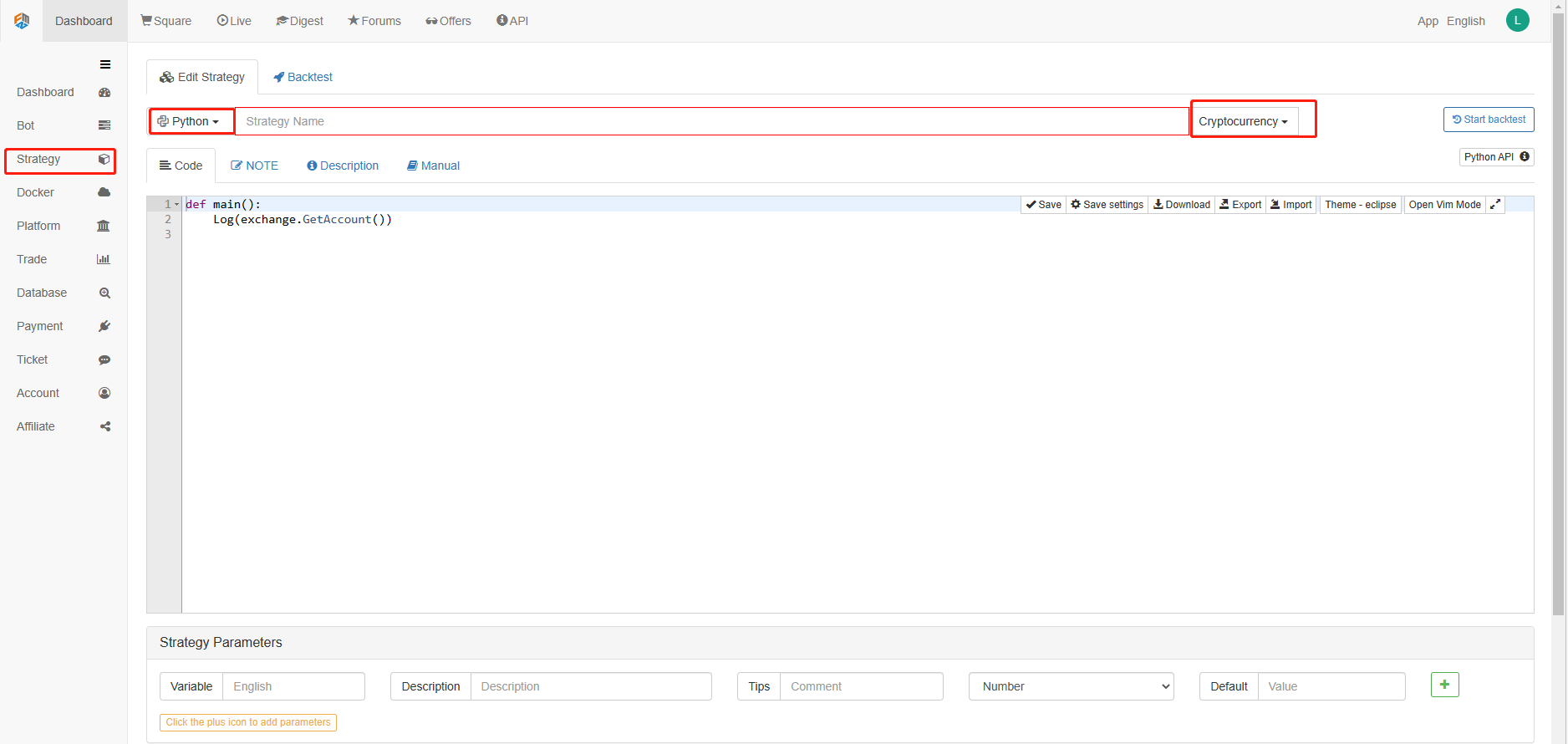
Ensuite, nous allons écrire du code Python dans la page d'édition du code.
Nous utiliserons les contrats à terme OKCoin pour tester la stratégie:
import time # Here we need to introduce the time library that comes with python, which will be used later in the program.

class Error_noSupport(BaseException): # We define a global class named ChartCfg to initialize the strategy chart settings. Object has many attributes about the chart function. Chart library: HighCharts.
    def __init__(self): # log out prompt messages
        Log("Support OKCoin Futures only! #FF0000")

class Error_AtBeginHasPosition(BaseException):
    def __init__(self):
        Log("Start with a futures position! #FF0000")

ChartCfg = {
    '__isStock': True, # This attribute is used to control whether to display a single control data series (you can cancel the display of a single data series on the chart). If you specify __isStock: false, it will be displayed as a normal chart.
    'title': { # title is the main title of the chart
        'text': 'Dual Thrust upper and bottom track chart' # An attribute of the title text is the text of the title, here set to 'Dual Thrust upper and bottom track chart' the text will be displayed in the title position.
    },
    'yAxis': { # Settings related to the Y-axis of the chart coordinate.
        'plotLines': [{ # Horizontal lines on the Y-axis (perpendicular to the Y-axis), the value of this attribute is an array, i.e. the setting of multiple horizontal lines.
            'value': 0, # Coordinate value of horizontal line on Y-axis
            'color': 'red', # Color of horizontal line
            'width': 2, # Line width of horizontal line
            'label': {  # Labels on the horizontal line
                'text': 'Upper track', # Text of the label
                'align': 'center' # The display position of the label, here set to center (i.e.: 'center')
            },
        }, {       # The second horizontal line ([{...} , {...}] the second element in the array)
            'value': 0, # Coordinate value of horizontal line on Y-axis
            'color': 'green', # Color of horizontal line
            'width': 2,  # Line width of horizontal line
            'label': { # Label
                'text': 'bottom track',
                'align': 'center'
            },
        }]
    },
    'series': [{ # Data series, that is, data used to display data lines, K-lines, tags, and other contents on the chart. It is also an array whose first index is 0.
        'type': 'candlestick', # Type of data series with index 0: 'candlestick' indicates a K-line chart.
        'name': 'Current period',  # Name of the data series
        'id': 'primary', # The ID of the data series, which is used for the related settings of the next data series.
        'data': []  # An array of data series to store specific K-line data
    }, {
        'type': 'flags',  # Data series, type: 'flags', display labels on the chart, indicating going long and going short. Index is 1.
        'onSeries': 'primary',  # This attribute indicates that the label is displayed on id 'primary'.
        'data': []    # The array that holds the label data.
    }]
}

STATE_IDLE = 0  # Status constants, indicating idle
STATE_LONG = 1 # Status constants, indicating long positions
STATE_SHORT = 2 # Status constants, indicating short positions
State = STATE_IDLE # Indicates the current program status, assigned as idle initially

LastBarTime = 0  # The time stamp of the last column of the K-line (in milliseconds, 1000 milliseconds is equal to 1 second, and the timestamp is the number of milliseconds from January 1, 1970 to the present time is a large positive integer).
UpTrack = 0   # Upper track value
BottomTrack = 0 # Bottom track value
chart = None # It is used to accept the chart control object returned by the Chart API function. Use this object (chart) to call its member function to write data to the chart.
InitAccount = None # Initial account status
LastAccount = None # Latest account status
Counter = { # Counters for recording profit and loss counts
    'w': 0, # Number of wins
    'l': 0  # Number of losses
}

def GetPosition(posType):  # Define a function to store account position information
    positions = exchange.GetPosition() # exchange.GetPosition() is the FMZ Quant official API. For its usage, please refer to the official API document: https://www.fmz.com/api.
    return [{'Price': position['Price'], 'Amount': position['Amount']} for position in positions if position['Type'] == posType] # Return to various position information

def CancelPendingOrders(): # Define a function specifically for withdrawing orders
    while True: # Loop check
        orders = exchange.GetOrders() # If there is a position
        [exchange.CancelOrder(order['Id']) for order in orders if not Sleep(500)] # Withdrawal statement
        if len(orders) == 0: # Logical judgment
            break

def Trade(currentState,nextState): # Define a function to determine the order placement logic.
    global InitAccount,LastAccount,OpenPrice,ClosePrice # Define the global scope
    ticker = _C(exchange.GetTicker) # For the usage of _C, please refer to: https://www.fmz.com/api.
    slidePrice = 1 # Define the slippage value
    pfn = exchange.Buy if nextState == STATE_LONG else exchange.Sell # Buying and selling judgment logic
    if currentState != STATE_IDLE: # Loop start
        Log(_C(exchange.GetPosition)) # Log information
        exchange.SetDirection("closebuy" if currentState == STATE_LONG else "closesell") # Adjust the order direction, especially after placing the order.
        while True:
            ID = pfn( (ticker['Last'] - slidePrice) if currentState == STATE_LONG else (ticker['Last'] + slidePrice), AmountOP) # Price limit order, ID=pfn (- 1, AmountOP) is the market price order, ID=pfn (AmountOP) is the market price order.
            Sleep(Interval) # Take a break to prevent the API from being accessed too often and your account being blocked.
            Log(exchange.GetOrder(ID)) # Log information
            ClosePrice = (exchange.GetOrder(ID))['AvgPrice'] # Set the closing price
            CancelPendingOrders() # Call the withdrawal function
            if len(GetPosition(PD_LONG if currentState == STATE_LONG else PD_SHORT)) == 0: # Order withdrawal logic
                break
        account = exchange.GetAccount() # Get account information
        if account['Stocks'] > LastAccount['Stocks']: # If the current account currency value is greater than the previous account currency value.
            Counter['w'] += 1 # In the profit and loss counter, add one to the number of profits.
        else:
            Counter['l'] += 1 # Otherwise, add one to the number of losses.
        Log(account) # log information
        LogProfit((account['Stocks'] - InitAccount['Stocks']),"Return rates:", ((account['Stocks'] - InitAccount['Stocks']) * 100 / InitAccount['Stocks']),'%')
        Cal(OpenPrice,ClosePrice)
        LastAccount = account

    exchange.SetDirection("buy" if nextState == STATE_LONG else "sell") # The logic of this part is the same as above and will not be elaborated.
    Log(_C(exchange.GetAccount))
    while True:
        ID = pfn( (ticker['Last'] + slidePrice) if nextState == STATE_LONG else (ticker['Last'] - slidePrice), AmountOP)
        Sleep(Interval)
        Log(exchange.GetOrder(ID))
        CancelPendingOrders()
        pos = GetPosition(PD_LONG if nextState == STATE_LONG else PD_SHORT)
        if len(pos) != 0:
            Log("Average price of positions",pos[0]['Price'],"Amount:",pos[0]['Amount'])
            OpenPrice = (exchange.GetOrder(ID))['AvgPrice']
            Log("now account:",exchange.GetAccount())
            break

def onTick(exchange): # The main function of the program, within which the main logic of the program is processed.
    global LastBarTime,chart,State,UpTrack,DownTrack,LastAccount # Define the global scope
    records = exchange.GetRecords() # For the usage of exchange.GetRecords(), please refer to: https://www.fmz.com/api.
    if not records or len(records) <= NPeriod: # Judgment statements to prevent accidents.
        return
    Bar = records[-1] # Take the penultimate element of records K-line data, that is, the last bar.
    if LastBarTime != Bar['Time']:
        HH = TA.Highest(records, NPeriod, 'High')  # Declare the HH variable, call the TA.Highest function to calculate the maximum value of the highest price in the current K-line data NPeriod period and assign it to HH.
        HC = TA.Highest(records, NPeriod, 'Close') # Declare the HC variable to get the maximum value of the closing price in the NPeriod period.
        LL = TA.Lowest(records, NPeriod, 'Low') # Declare the LL variable to get the minimum value of the lowest price in the NPeriod period.
        LC = TA.Lowest(records, NPeriod, 'Close') # Declare LC variable to get the minimum value of the closing price in the NPeriod period. For specific TA-related applications, please refer to the official API documentation.

        Range = max(HH - LC, HC - LL)  # Calculate the range
        UpTrack = _N(Bar['Open'] + (Ks * Range))  # The upper track value is calculated based on the upper track factor Ks of the interface parameters such as the opening price of the latest K-line bar.
        DownTrack = _N(Bar['Open'] - (Kx * Range)) # Calculate the down track value
        if LastBarTime > 0: # Because the value of LastBarTime initialization is set to 0, LastBarTime>0 must be false when running here for the first time. The code in the if block will not be executed, but the code in the else block will be executed.
            PreBar = records[-2] # Declare a variable means "the previous Bar" assigns the value of the penultimate Bar of the current K-line to it.
            chart.add(0, [PreBar['Time'], PreBar['Open'], PreBar['High'], PreBar['Low'], PreBar['Close']], -1) # Call the add function of the chart icon control class to update the K-line data (use the penultimate bar of the obtained K-line data to update the last bar of the icon, because a new K-line bar is generated).
        else:  # For the specific usage of the chart.add function, see the API documentation and the articles in the forum. When the program runs for the first time, it must execute the code in the else block. The main function is to add all the K-lines obtained for the first time to the chart at one time.
            for i in range(len(records) - min(len(records), NPeriod * 3), len(records)): # Here, a for loop is executed. The number of loops uses the minimum of the K-line length and 3 times the NPeriod, which can ensure that the initial K-line will not be drawn too much and too long. Indexes vary from large to small.
                b = records[i] # Declare a temporary variable b to retrieve the K-line bar data with the index of records.length - i for each loop.
                chart.add(0,[b['Time'], b['Open'], b['High'], b['Low'], b['Close']]) # Call the chart.add function to add a K-line bar to the chart. Note that if the last parameter of the add function is passed in -1, it will update the last Bar (column) on the chart. If no parameter is passed in, it will add Bar to the last. After executing the loop of i=2 (i-- already, now it's 1), it will trigger i > 1 for false to stop the loop. It can be seen that the code here only processes the bar of records.length - 2, and the last Bar is not processed.
        chart.add(0,[Bar['Time'], Bar['Open'], Bar['High'], Bar['Low'], Bar['Close']]) # Since the two branches of the above if do not process the bar of records.length - 1, it is processed here. Add the latest Bar to the chart.
        ChartCfg['yAxis']['plotLines'][0]['value'] = UpTrack  # Assign the calculated upper track value to the chart object (different from the chart control object chart) for later display.
        ChartCfg['yAxis']['plotLines'][1]['value'] = DownTrack # Assign lower track value
        ChartCfg['subtitle'] = { # Set subtitle
            'text': 'upper tarck' + str(UpTrack) + 'down track' + str(DownTrack) # Subtitle text setting. The upper and down track values are displayed on the subtitle.
        }
        chart.update(ChartCfg) # Update charts with chart class ChartCfg.
        chart.reset(PeriodShow) # Refresh the PeriodShow variable set according to the interface parameters, and only keep the K-line bar of the number of PeriodShow values.

        LastBarTime = Bar['Time'] # The timestamp of the newly generated Bar is updated to LastBarTime to determine whether the last Bar of the K-line data acquired in the next loop is a newly generated one.
    else: # If LastBarTime is equal to Bar.Time, that is, no new K-line Bar is generated. Then execute the code in {..}.
        chart.add(0,[Bar['Time'], Bar['Open'], Bar['High'], Bar['Low'], Bar['Close']], -1) # Update the last K-line bar on the chart with the last Bar of the current K-line data (the last Bar of the K-line, i.e. the Bar of the current period, is constantly changing).
    LogStatus("Price:", Bar["Close"], "up:", UpTrack, "down:", DownTrack, "wins:", Counter['w'], "losses:", Counter['l'], "Date:", time.time()) # The LogStatus function is called to display the data of the current strategy on the status bar.
    msg = "" # Define a variable msg.
    if State == STATE_IDLE or State == STATE_SHORT: # Judge whether the current state variable State is equal to idle or whether State is equal to short position. In the idle state, it can trigger long position, and in the short position state, it can trigger a long position to be closed and sell the opening position.
        if Bar['Close'] >= UpTrack: # If the closing price of the current K-line is greater than the upper track value, execute the code in the if block.
            msg = "Go long, trigger price:" + str(Bar['Close']) + "upper track" + str(UpTrack) # Assign a value to msg and combine the values to be displayed into a string.
            Log(msg) # message
            Trade(State, STATE_LONG) # Call the Trade function above to trade.
            State = STATE_LONG # Regardless of opening long positions or selling the opening position, the program status should be updated to hold long positions at the moment.
            chart.add(1,{'x': Bar['Time'], 'color': 'red', 'shape': 'flag', 'title': 'long', 'text': msg}) # Add a marker to the corresponding position of the K-line to show the open long position.

    if State == STATE_IDLE or State == STATE_LONG: # The short direction is the same as the above, and will not be repeated. The code is exactly the same.
        if Bar['Close'] <= DownTrack:
            msg = "Go short, trigger price:" + str(Bar['Close']) + "down track" + str(DownTrack)
            Log(msg)
            Trade(State, STATE_SHORT)
            State = STATE_SHORT
            chart.add(1,{'x': Bar['Time'], 'color': 'green', 'shape': 'circlepin', 'title': 'short', 'text': msg})

OpenPrice = 0 # Initialize OpenPrice and ClosePrice
ClosePrice = 0
def Cal(OpenPrice, ClosePrice): # Define a Cal function to calculate the profit and loss of the strategy after it has been run.
    global AmountOP,State
    if State == STATE_SHORT:
        Log(AmountOP,OpenPrice,ClosePrice,"Profit and loss of the strategy:", (AmountOP * 100) / ClosePrice - (AmountOP * 100) / OpenPrice, "Currencies, service charge:", - (100 * AmountOP * 0.0003), "USD, equivalent to:", _N( - 100 * AmountOP * 0.0003/OpenPrice,8), "Currencies")
        Log(((AmountOP * 100) / ClosePrice - (AmountOP * 100) / OpenPrice) + (- 100 * AmountOP * 0.0003/OpenPrice))
    if State == STATE_LONG:
        Log(AmountOP,OpenPrice,ClosePrice,"Profit and loss of the strategy:", (AmountOP * 100) / OpenPrice - (AmountOP * 100) / ClosePrice, "Currencies, service charge:", - (100 * AmountOP * 0.0003), "USD, equivalent to:", _N( - 100 * AmountOP * 0.0003/OpenPrice,8), "Currencies")
        Log(((AmountOP * 100) / OpenPrice - (AmountOP * 100) / ClosePrice) + (- 100 * AmountOP * 0.0003/OpenPrice))

def main(): # The main function of the strategy program. (entry function)
    global LoopInterval,chart,LastAccount,InitAccount # Define the global scope
    if exchange.GetName() != 'Futures_OKCoin':  # Judge if the name of the added exchange object (obtained by the exchange.GetName function) is not equal to 'Futures_OKCoin', that is, the object added is not OKCoin futures exchange object.
        raise Error_noSupport # Throw an exception
    exchange.SetRate(1) # Set various parameters of the exchange.
    exchange.SetContractType(["this_week","next_week","quarter"][ContractTypeIdx])  # Determine which specific contract to trade.
    exchange.SetMarginLevel([10,20][MarginLevelIdx]) # Set the margin rate, also known as leverage.

    if len(exchange.GetPosition()) > 0: # Set up fault tolerance mechanism.
        raise Error_AtBeginHasPosition
    CancelPendingOrders()
    InitAccount = LastAccount = exchange.GetAccount()
    LoopInterval = min(1,LoopInterval)
    Log("Trading platforms:",exchange.GetName(), InitAccount)
    LogStatus("Ready...")

    LogProfitReset()
    chart = Chart(ChartCfg)
    chart.reset()

    LoopInterval = max(LoopInterval, 1)
    while True: # Loop the whole transaction logic and call the onTick function.
        onTick(exchange)
        Sleep(LoopInterval * 1000) # Take a break to prevent the API from being accessed too frequently and the account from being blocked.
Après avoir écrit le code, veuillez noter que nous n'avons pas terminé toute la stratégie. Ensuite, nous devons ajouter les paramètres utilisés dans la stratégie à la page d'édition de la stratégie. La méthode d'ajout est très simple. Cliquez simplement sur le signe plus en bas de la boîte de dialogue de rédaction de stratégie pour ajouter un par un.
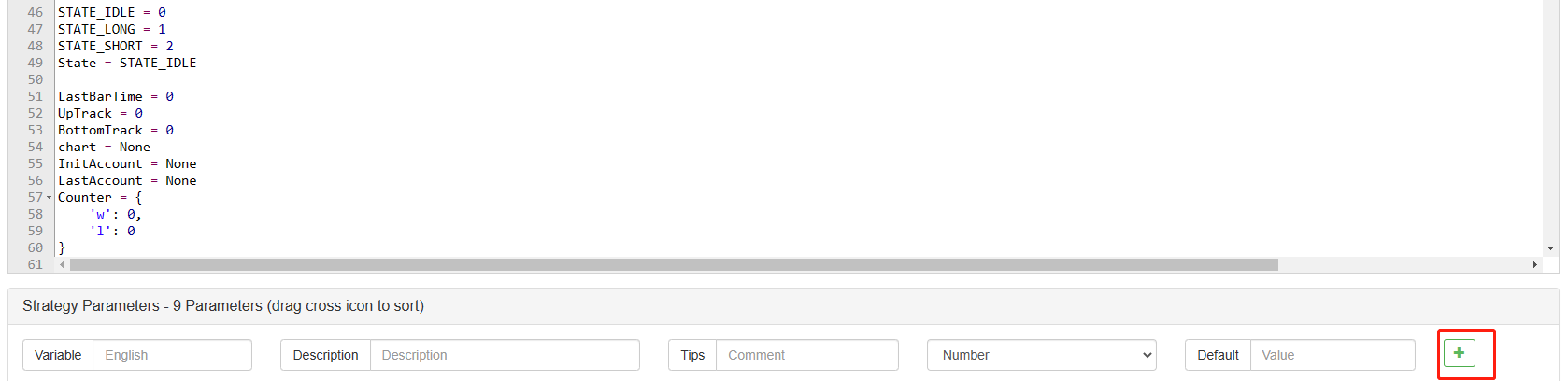
Contenu à ajouter:
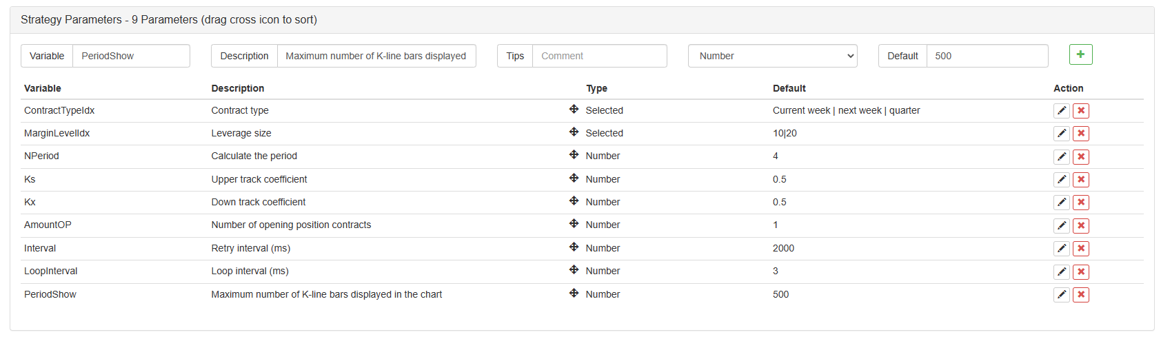
Pour l'instant, nous avons finalement terminé la rédaction de la stratégie.
Tests antérieurs de stratégie
Après avoir écrit la stratégie, la première chose que nous devons faire est de la backtest pour voir comment elle se comporte dans les données historiques. Mais veuillez noter que le résultat du backtest n'est pas égal à la prédiction de l'avenir. Le backtest ne peut être utilisé que comme référence pour considérer l'efficacité de notre stratégie. Une fois que le marché change et que la stratégie commence à avoir de grandes pertes, nous devons trouver le problème à temps, puis changer la stratégie pour nous adapter au nouvel environnement du marché, comme le seuil mentionné ci-dessus. Si la stratégie a une perte supérieure à 10%, nous devons immédiatement arrêter le fonctionnement de la stratégie, puis trouver le problème. Nous pouvons commencer par ajuster le seuil.
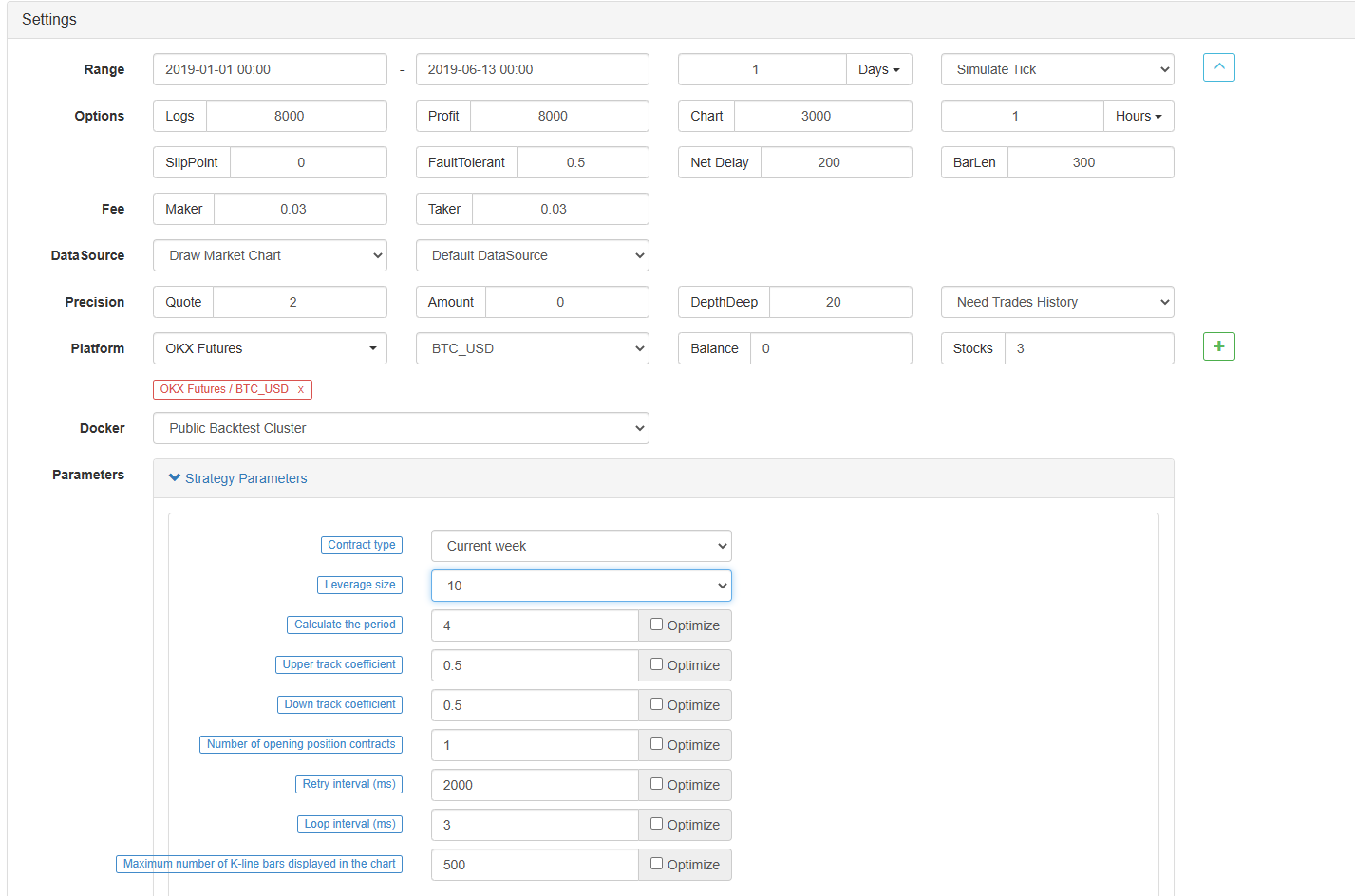
Cliquez sur backtest dans la page d'édition de la stratégie. Sur la page de backtest, l'ajustement des paramètres peut être effectué de manière pratique et rapide en fonction des différents besoins. Surtout pour la stratégie avec une logique complexe et de nombreux paramètres, il n'est pas nécessaire de revenir au code source et de le modifier un par un.
Le temps de backtest est les six derniers mois. Cliquez sur Ajouter l'échange OKCoin Futures et sélectionnez la cible de trading BTC.
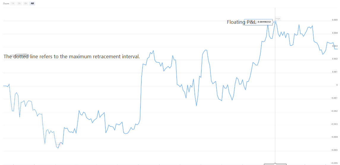
On peut voir que la stratégie a récolté de bons rendements au cours des six derniers mois en raison de la très bonne tendance unilatérale de BTC.

Si vous avez des questions, vous pouvez laisser un message à:https://www.fmz.com/bbs, qu'il s'agisse de la stratégie ou de la technologie de la plateforme, la plateforme FMZ Quant dispose de professionnels prêts à répondre à vos questions.
- Quantifier l'analyse fondamentale sur le marché des crypto-monnaies: laissez les données parler d'elles-mêmes!
- Les fondements de la recherche quantifiée dans le cercle monétaire - ne croyez plus à tous les professeurs de mathématiques, les données sont objectives!
- Un outil indispensable dans le domaine de la quantification des transactions - l'inventeur du module de recherche de données quantifiées
- Maîtriser tout - Introduction à FMZ Nouvelle version du terminal de négociation (avec le code source TRB Arbitrage)
- Tout savoir sur la nouvelle version du terminal de trading FMZ (source code TRB)
- FMZ Quant: Une analyse des exemples de conception des exigences communes sur le marché des crypto-monnaies (II)
- Comment exploiter les robots de vente sans cerveau avec une stratégie de haute fréquence en 80 lignes de code
- Quantification FMZ: analyse de l'exemple de conception des besoins courants sur le marché des crypto-monnaies (II)
- Comment exploiter les robots sans cerveau pour les vendre avec une stratégie de haute fréquence de 80 lignes de code
- FMZ Quant: Une analyse des exemples de conception des exigences communes sur le marché des crypto-monnaies (I)
- Quantification FMZ: analyse de l'exemple de conception des besoins courants sur le marché des crypto-monnaies (1)