

본 논문에서는 주로 고빈도 거래 전략에 대해 논의하며, 누적 거래량 모델링과 가격 충격에 초점을 맞추고 있습니다. 본 논문에서는 단일 거래, 고정 간격 가격 충격, 거래량이 가격에 미치는 영향을 분석하여 예비적 최적 주문 배치 모델을 제안한다. 이 모델은 거래량과 가격 충격에 대한 이해를 바탕으로 최적의 거래 포지션을 찾으려고 시도합니다. 모델의 가정에 대해 심도 있게 논의하며, 실제 수익과 모델에서 예측한 기대 수익을 비교하여 최적의 주문 배치에 대한 예비 평가가 이루어집니다.
누적 볼륨 모델링
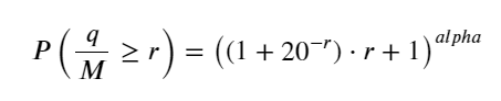
이전 기사에서는 단일 거래량이 특정 값보다 클 확률 표현식을 도출했습니다.
우리는 또한 특정 기간에 걸친 거래량의 분포에 대해서도 우려하고 있는데, 이는 직관적으로 각 거래량과 주문 빈도와 관련이 있어야 합니다. 다음으로, 데이터는 고정된 간격으로 처리됩니다. 위와 같이 분포를 표시하세요.
python
from datetime import date,datetime
import time
import pandas as pd
import numpy as np
import matplotlib.pyplot as plt
%matplotlib inline
            python

            trades = pd.read_csv('HOOKUSDT-aggTrades-2023-01-27.csv')
trades['date'] = pd.to_datetime(trades['transact_time'], unit='ms')
trades.index = trades['date']
buy_trades = trades[trades['is_buyer_maker']==False].copy()
buy_trades = buy_trades.groupby('transact_time').agg({
    'agg_trade_id': 'last',
    'price': 'last',
    'quantity': 'sum',
    'first_trade_id': 'first',
    'last_trade_id': 'last',
    'is_buyer_maker': 'last',
    'date': 'last',
    'transact_time':'last'
})
buy_trades['interval']=buy_trades['transact_time'] - buy_trades['transact_time'].shift()
buy_trades.index = buy_trades['date']
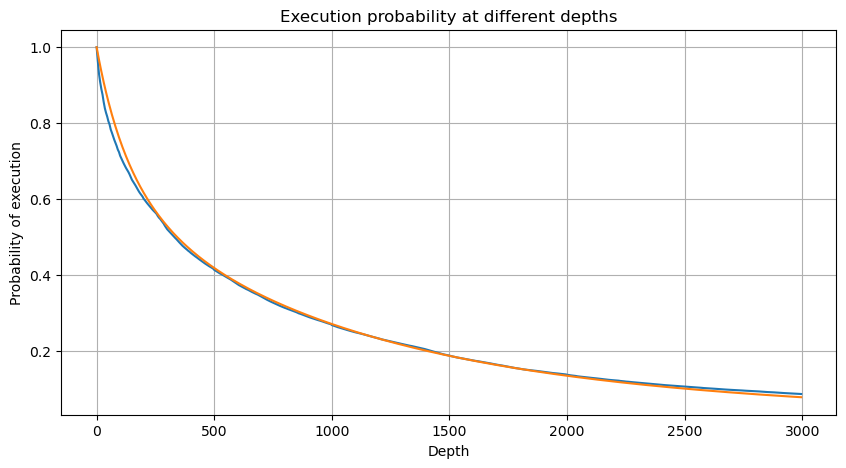
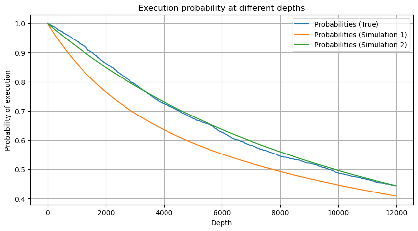
1초마다 거래량을 합치고, 거래가 발생하지 않은 부분을 제거하고, 위의 단일 거래의 분포를 사용하여 맞추면 결과가 더 좋아지는 것을 알 수 있다. 1초 내의 모든 거래를 단일 거래로 간주하면 이 문제는 다음과 같다. 해결된 문제가 되었습니다. 그러나 주기가 길어지면(거래 빈도에 비해) 오류가 증가하는 것으로 나타났으며, 연구에 따르면 이 오류는 이전 파레토 분포 수정 항목으로 인해 발생한다는 것이 밝혀졌습니다. 즉, 사이클이 길어지고 개별 거래가 더 많아질수록 여러 거래의 조합이 파레토 분포에 접근합니다. 이 경우 수정 항을 제거해야 합니다.
            python

            df_resampled = buy_trades['quantity'].resample('1S').sum()
df_resampled = df_resampled.to_frame(name='quantity')
df_resampled = df_resampled[df_resampled['quantity']>0]
            python

            buy_trades
| agg_trade_id | price | quantity | first_trade_id | last_trade_id | is_buyer_maker | date | transact_time | interval | diff | |
|---|---|---|---|---|---|---|---|---|---|---|
| 2023-01-27 00:00:00.161 | 1138369 | 2.901 | 54.3 | 3806199 | 3806201 | False | 2023-01-27 00:00:00.161 | 1674777600161 | NaN | 0.001 |
| 2023-01-27 00:00:04.140 | 1138370 | 2.901 | 291.3 | 3806202 | 3806203 | False | 2023-01-27 00:00:04.140 | 1674777604140 | 3979.0 | 0.000 |
| 2023-01-27 00:00:04.339 | 1138373 | 2.902 | 55.1 | 3806205 | 3806207 | False | 2023-01-27 00:00:04.339 | 1674777604339 | 199.0 | 0.001 |
| 2023-01-27 00:00:04.772 | 1138374 | 2.902 | 1032.7 | 3806208 | 3806223 | False | 2023-01-27 00:00:04.772 | 1674777604772 | 433.0 | 0.000 |
| 2023-01-27 00:00:05.562 | 1138375 | 2.901 | 3.5 | 3806224 | 3806224 | False | 2023-01-27 00:00:05.562 | 1674777605562 | 790.0 | 0.000 |
| ... | ... | ... | ... | ... | ... | ... | ... | ... | ... | ... |
| 2023-01-27 23:59:57.739 | 1544370 | 3.572 | 394.8 | 5074645 | 5074651 | False | 2023-01-27 23:59:57.739 | 1674863997739 | 1224.0 | 0.002 |
| 2023-01-27 23:59:57.902 | 1544372 | 3.573 | 177.6 | 5074652 | 5074655 | False | 2023-01-27 23:59:57.902 | 1674863997902 | 163.0 | 0.001 |
| 2023-01-27 23:59:58.107 | 1544373 | 3.573 | 139.8 | 5074656 | 5074656 | False | 2023-01-27 23:59:58.107 | 1674863998107 | 205.0 | 0.000 |
| 2023-01-27 23:59:58.302 | 1544374 | 3.573 | 60.5 | 5074657 | 5074657 | False | 2023-01-27 23:59:58.302 | 1674863998302 | 195.0 | 0.000 |
| 2023-01-27 23:59:59.894 | 1544376 | 3.571 | 12.1 | 5074662 | 5074664 | False | 2023-01-27 23:59:59.894 | 1674863999894 | 1592.0 | 0.000 |
            python

            #1s内的累计分布
depths = np.array(range(0, 3000, 5))
probabilities = np.array([np.mean(df_resampled['quantity'] > depth) for depth in depths])
mean = df_resampled['quantity'].mean()
alpha = np.log(np.mean(df_resampled['quantity'] > mean))/np.log(2.05)
probabilities_s = np.array([((1+20**(-depth/mean))*depth/mean+1)**(alpha) for depth in depths])

plt.figure(figsize=(10, 5))
plt.plot(depths, probabilities)
plt.plot(depths, probabilities_s)
plt.xlabel('Depth')
plt.ylabel('Probability of execution')
plt.title('Execution probability at different depths')
plt.grid(True)
            python

            df_resampled = buy_trades['quantity'].resample('30S').sum()
df_resampled = df_resampled.to_frame(name='quantity')
df_resampled = df_resampled[df_resampled['quantity']>0]
depths = np.array(range(0, 12000, 20))
probabilities = np.array([np.mean(df_resampled['quantity'] > depth) for depth in depths])
mean = df_resampled['quantity'].mean()
alpha = np.log(np.mean(df_resampled['quantity'] > mean))/np.log(2.05)
probabilities_s = np.array([((1+20**(-depth/mean))*depth/mean+1)**(alpha) for depth in depths])
alpha = np.log(np.mean(df_resampled['quantity'] > mean))/np.log(2)
probabilities_s_2 = np.array([(depth/mean+1)**alpha for depth in depths]) # 无修正

plt.figure(figsize=(10, 5))
plt.plot(depths, probabilities,label='Probabilities (True)')
plt.plot(depths, probabilities_s, label='Probabilities (Simulation 1)')
plt.plot(depths, probabilities_s_2, label='Probabilities (Simulation 2)')
plt.xlabel('Depth')
plt.ylabel('Probability of execution')
plt.title('Execution probability at different depths')
plt.legend()
plt.grid(True)
이제 우리는 다양한 시간대별 누적 거래량 분포에 대한 일반 공식을 요약하고, 이를 맞추기 위해 개별 거래량의 분포를 사용했으며, 매번 개별적으로 계산할 필요가 없었습니다. 여기에서는 과정을 생략하고 공식을 직접 제시합니다.
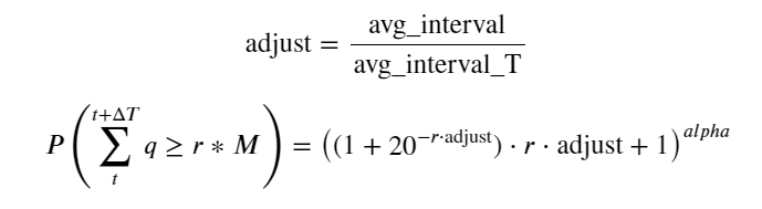
그 중 avg_interval은 단일 거래 간의 평균 간격을 나타내고, avg_interval_T는 추정해야 할 간격의 평균 간격을 나타냅니다. 약간 혼란스럽습니다. 1초의 거래 시간을 추정하려면 1초 내에 거래가 포함된 이벤트 간의 평균 간격을 계산해야 합니다. 주문이 도착할 확률이 포아송 분포를 따른다면 여기서 직접 추정하는 것이 가능해야 하지만, 실제 편차가 크기 때문에 여기서는 설명하지 않겠습니다.
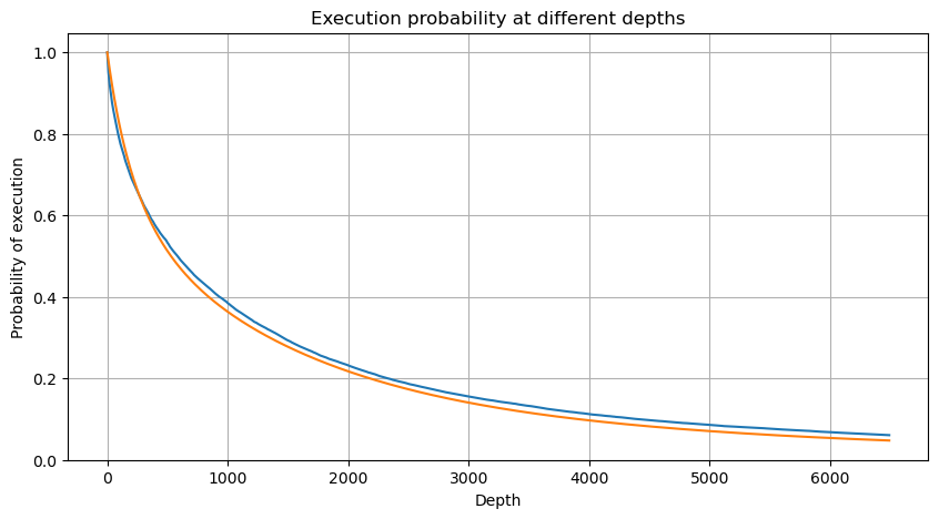
특정 간격 내에서 특정 값보다 큰 볼륨의 확률은 깊이의 해당 위치에서 거래의 실제 확률과 상당히 달라야 합니다. 대기 시간이 길수록 주문장이 체결될 가능성이 커지기 때문입니다. 변경되고, 거래도 깊이로 이어집니다. 따라서 동일한 깊이 위치에서의 거래 확률은 데이터가 업데이트됨에 따라 실시간으로 변경됩니다.
            python

            df_resampled = buy_trades['quantity'].resample('2S').sum()
df_resampled = df_resampled.to_frame(name='quantity')
df_resampled = df_resampled[df_resampled['quantity']>0]
depths = np.array(range(0, 6500, 10))
probabilities = np.array([np.mean(df_resampled['quantity'] > depth) for depth in depths])
mean = buy_trades['quantity'].mean()
adjust = buy_trades['interval'].mean() / 2620
alpha = np.log(np.mean(buy_trades['quantity'] > mean))/0.7178397931503168
probabilities_s = np.array([((1+20**(-depth*adjust/mean))*depth*adjust/mean+1)**(alpha) for depth in depths])

plt.figure(figsize=(10, 5))
plt.plot(depths, probabilities)
plt.plot(depths, probabilities_s)
plt.xlabel('Depth')
plt.ylabel('Probability of execution')
plt.title('Execution probability at different depths')
plt.grid(True)
단일 거래 가격 영향
거래 데이터는 귀중한 보물이며, 아직도 채굴되어야 할 데이터가 많이 있습니다. 우리는 전략에 따른 보류 주문의 배치에 영향을 미치는 가격에 대한 주문의 영향에 주의를 기울여야 합니다. 마찬가지로 transact_time 집계 데이터를 기반으로 마지막 가격과 첫 번째 가격의 차이를 계산합니다. 주문이 하나뿐인 경우 차이는 0입니다. 이상한 점은 여전히 부정적인 결과가 있는 데이터 결과가 소수 있다는 것입니다. 이는 데이터 배열 순서에 문제가 있을 것이므로 여기서는 다루지 않겠습니다.
결과에 따르면 영향 없음 비율은 최대 77%, 1틱 비율은 16.5%, 2틱 비율은 3.7%, 3틱 비율은 1.2%, 4틱 이상 비율은 1% 미만으로 나타났다. . 이는 기본적으로 지수 함수의 특성과 일치하지만 적합성이 정확하지 않습니다.
해당 가격 차이를 발생시킨 거래량을 계산하고 충격이 너무 커서 발생한 왜곡을 제거했습니다. 기본적으로 선형 관계에 부합하며, 약 1,000 볼륨마다 1틱의 가격 변동이 발생합니다. 각 가격 근처의 보류 주문 평균 수는 약 1,000개라는 것을 알 수 있습니다.
            python

            diff_df = trades[trades['is_buyer_maker']==False].groupby('transact_time')['price'].agg(lambda x: abs(round(x.iloc[-1] - x.iloc[0],3)) if len(x) > 1 else 0)
buy_trades['diff'] = buy_trades['transact_time'].map(diff_df)
            python

            diff_counts = buy_trades['diff'].value_counts()
diff_counts[diff_counts>10]/diff_counts.sum()
            0.000    0.769965
0.001    0.165527
0.002    0.037826
0.003    0.012546
0.004    0.005986
0.005    0.003173
0.006    0.001964
0.007    0.001036
0.008    0.000795
0.009    0.000474
0.010    0.000227
0.011    0.000187
0.012    0.000087
0.013    0.000080
Name: diff, dtype: float64
            python

            diff_group = buy_trades.groupby('diff').agg({
    'quantity': 'mean',
    'diff': 'last',
})
            python

            diff_group['quantity'][diff_group['diff']>0][diff_group['diff']<0.01].plot(figsize=(10,5),grid=True);
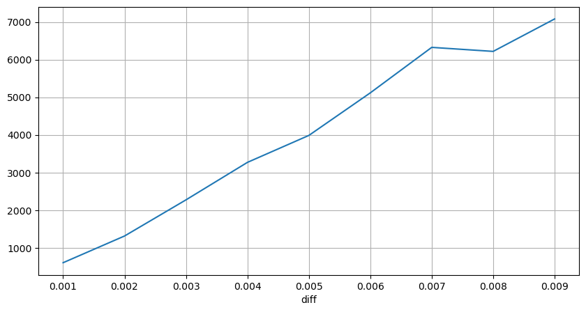
정기적으로 가격 충격이 발생합니다.
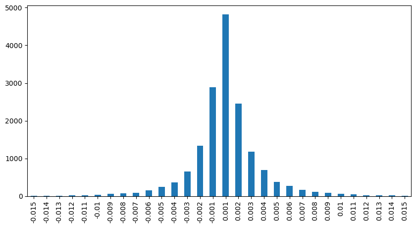
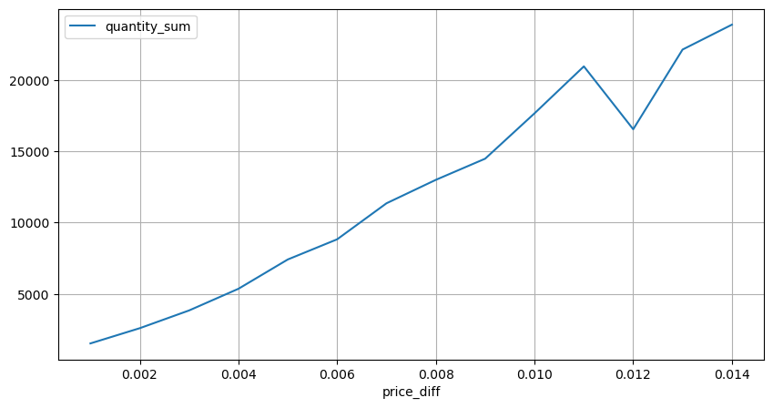
2초 이내에 가격 영향을 계산합니다. 여기서 차이점은 음수 값이 있다는 것입니다. 물론, 여기서는 매수 주문만 계산되므로 대칭적 위치는 1틱 더 큽니다. 거래량과 영향 사이의 관계를 계속 관찰하고 0보다 큰 결과만 계산합니다. 결론은 단일 주문의 결론과 유사하며, 이는 또한 대략적인 선형 관계입니다. 각 틱에는 약 2000 볼륨이 필요합니다.
            python

            df_resampled = buy_trades.resample('2S').agg({
    'price': ['first', 'last', 'count'],
    'quantity': 'sum'
})
df_resampled['price_diff'] = round(df_resampled[('price', 'last')] - df_resampled[('price', 'first')],3)
df_resampled['price_diff'] = df_resampled['price_diff'].fillna(0)
result_df_raw = pd.DataFrame({
    'price_diff': df_resampled['price_diff'],
    'quantity_sum': df_resampled[('quantity', 'sum')],
    'data_count': df_resampled[('price', 'count')]
})
result_df = result_df_raw[result_df_raw['price_diff'] != 0]
            python

            result_df['price_diff'][abs(result_df['price_diff'])<0.016].value_counts().sort_index().plot.bar(figsize=(10,5));
            python

            result_df['price_diff'].value_counts()[result_df['price_diff'].value_counts()>30]
             0.001    7176
-0.001    3665
 0.002    3069
-0.002    1536
 0.003    1260
 0.004     692
-0.003     608
 0.005     391
-0.004     322
 0.006     259
-0.005     192
 0.007     146
-0.006     112
 0.008      82
 0.009      75
-0.007      75
-0.008      65
 0.010      51
 0.011      41
-0.010      31
Name: price_diff, dtype: int64
            python

            diff_group = result_df.groupby('price_diff').agg({ 'quantity_sum': 'mean'})
            python

            diff_group[(diff_group.index>0) & (diff_group.index<0.015)].plot(figsize=(10,5),grid=True);
볼륨의 가격 영향
진드기 변화에 필요한 볼륨은 이전에 계산되었지만 충격이 이미 발생했다는 가정에 기초하고 있기 때문에 정확하지 않습니다. 이제 거래량에 따른 가격 영향을 살펴보겠습니다.
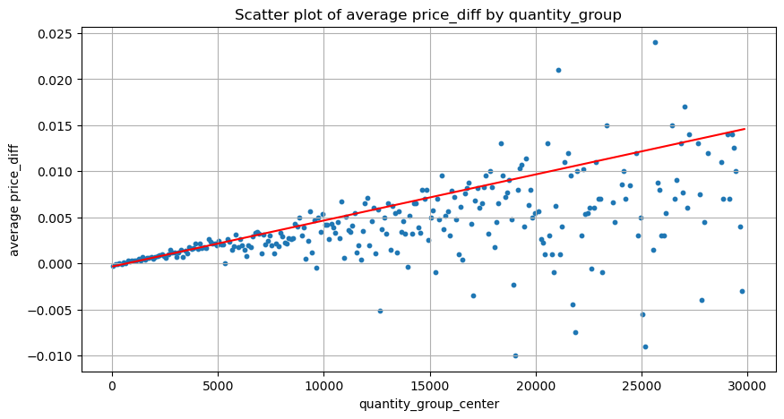
여기의 데이터는 1초마다 샘플링되며, 100개의 수량을 1단계로 하고, 이 수량 범위 내에서의 가격 변화가 계산됩니다. 몇 가지 귀중한 결론이 도출되었습니다.
- 매수량이 500 미만이면 예상 가격 변동이 낮아지는데, 이는 가격에 영향을 미치는 매도 주문도 있기 때문에 예상된 일입니다.
- 거래량이 낮을 때는 선형 관계를 따릅니다. 즉, 거래량이 클수록 가격 상승도 커집니다.
- 매수 주문량이 클수록 가격 변동이 커지는데, 이는 종종 가격 돌파를 나타냅니다. 돌파 후 가격이 돌아올 수 있습니다. 고정 간격으로 샘플링과 결합하면 데이터가 불안정합니다.
- 산점도의 윗부분, 즉 가격 상승에 상응하는 거래량이 있는 부분에 주의해야 합니다.
- 이 거래 쌍에 대해서만 볼륨과 가격 변화 간의 관계에 대한 대략적인 버전이 제공됩니다.
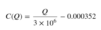
이 중 "C"는 가격 변화를 나타내고 "Q"는 매수 주문량을 나타냅니다.
            python

            df_resampled = buy_trades.resample('1S').agg({
    'price': ['first', 'last', 'count'],
    'quantity': 'sum'
})
df_resampled['price_diff'] = round(df_resampled[('price', 'last')] - df_resampled[('price', 'first')],3)
df_resampled['price_diff'] = df_resampled['price_diff'].fillna(0)
result_df_raw = pd.DataFrame({
    'price_diff': df_resampled['price_diff'],
    'quantity_sum': df_resampled[('quantity', 'sum')],
    'data_count': df_resampled[('price', 'count')]
})
result_df = result_df_raw[result_df_raw['price_diff'] != 0]
            python

            df = result_df.copy()
bins = np.arange(0, 30000, 100)  #
labels = [f'{i}-{i+100-1}' for i in bins[:-1]]
df.loc[:, 'quantity_group'] = pd.cut(df['quantity_sum'], bins=bins, labels=labels)
grouped = df.groupby('quantity_group')['price_diff'].mean()
            python

            grouped_df = pd.DataFrame(grouped).reset_index()
grouped_df['quantity_group_center'] = grouped_df['quantity_group'].apply(lambda x: (float(x.split('-')[0]) + float(x.split('-')[1])) / 2)

plt.figure(figsize=(10,5))
plt.scatter(grouped_df['quantity_group_center'], grouped_df['price_diff'],s=10)
plt.plot(grouped_df['quantity_group_center'], np.array(grouped_df['quantity_group_center'].values)/2e6-0.000352,color='red')
plt.xlabel('quantity_group_center')
plt.ylabel('average price_diff')
plt.title('Scatter plot of average price_diff by quantity_group')
plt.grid(True)
            python

            grouped_df.head(10)
| quantity_group | price_diff | quantity_group_center | |
|---|---|---|---|
| 0 | 0-199 | -0.000302 | 99.5 |
| 1 | 100-299 | -0.000124 | 199.5 |
| 2 | 200-399 | -0.000068 | 299.5 |
| 3 | 300-499 | -0.000017 | 399.5 |
| 4 | 400-599 | -0.000048 | 499.5 |
| 5 | 500-699 | 0.000098 | 599.5 |
| 6 | 600-799 | 0.000006 | 699.5 |
| 7 | 700-899 | 0.000261 | 799.5 |
| 8 | 800-999 | 0.000186 | 899.5 |
| 9 | 900-1099 | 0.000299 | 999.5 |
초기 최적 주문 위치
거래량 모델링과 가격 영향에 따른 거래량의 대략적인 모델을 통해 최적의 주문 위치를 계산할 수 있는 것으로 보입니다. 몇 가지 가정을 하고 무책임한 최적 가격 위치를 제시해 보겠습니다.
- 충격 후 가격이 원래 가치로 돌아간다고 가정합니다(물론 이는 가능성이 낮으며 충격 후 가격 변화에 대한 재분석이 필요합니다)
- 이 기간 동안 거래량과 주문 빈도의 분포가 사전 설정 요구 사항을 충족한다고 가정합니다(이 역시 부정확한데, 추정에 하루의 값이 사용되고 거래가 명백히 밀집되어 있기 때문입니다).
- 시뮬레이션 시간 동안 매도 주문이 단 한 건만 발생하고 그 후 포지션이 종료된다고 가정해 보겠습니다.
- 주문이 실행된 후, 특히 거래량이 매우 낮을 때 가격을 계속 끌어올릴 다른 매수 주문이 있다고 가정합니다. 이 효과는 여기서 무시되고 단순히 돌아올 것이라고 가정합니다.
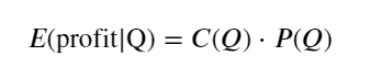
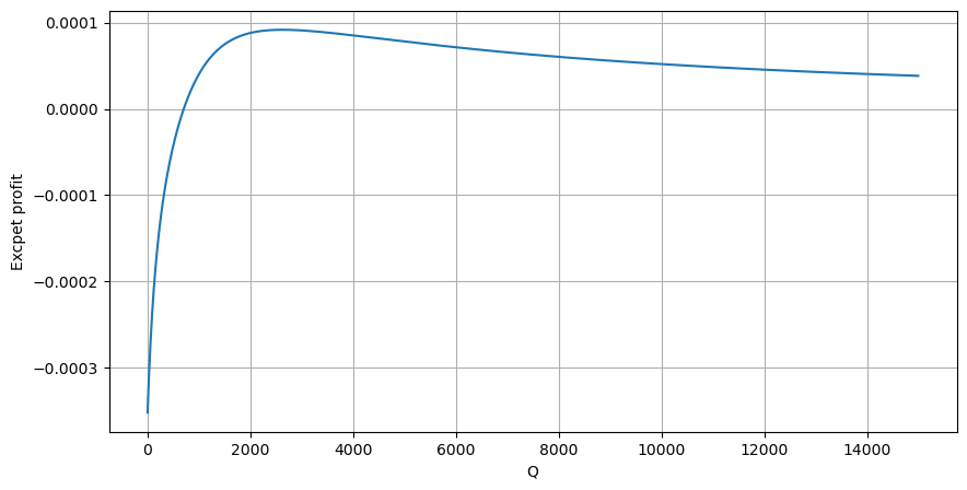
먼저 간단한 기대 수익률, 즉 누적 매수 주문이 1초 이내에 Q보다 클 확률에 기대 수익률(즉, 충격 가격)을 곱한 값을 작성합니다.
그래프에 따르면 기대 수익률은 약 2500에서 최대치를 보이며, 이는 평균 거래량의 약 2.5배입니다. 즉, 매도 주문은 2500에 해야 합니다. 수평축은 1초 내의 거래량을 나타내며, 단순히 깊이 위치와 동일시할 수 없다는 점을 다시 한번 강조할 필요가 있습니다. 그리고 이는 매우 중요한 심층적 데이터가 여전히 부족한 시점이며, 거래에 기초한 추측에 기초하고 있을 뿐입니다.
요약하다
다양한 시간 간격에서의 거래량 분포는 단일 거래의 거래량 분포를 간단히 나타낸 것임이 밝혀졌습니다. 또한 가격 충격과 거래 확률을 기반으로 간단한 기대 수익률 모델을 만들었습니다. 이 모델의 결과는 우리의 기대치와 일치합니다. 매도 주문량이 적으면 가격 하락을 나타냅니다. 수익을 내려면 일정 금액이 필요합니다. 마진이 크고 거래량이 많을수록 이익 마진이 높아집니다. 확률이 클수록 낮아집니다. 중간에 최적의 크기가 있는데, 이는 전략이 찾고 있는 주문 배치 위치이기도 합니다. 물론, 이 모델은 여전히 너무 단순합니다. 다음 글에서 계속해서 심도 있게 논의하겠습니다.
            python

            #1s内的累计分布
df_resampled = buy_trades['quantity'].resample('1S').sum()
df_resampled = df_resampled.to_frame(name='quantity')
df_resampled = df_resampled[df_resampled['quantity']>0]

depths = np.array(range(0, 15000, 10))
mean = df_resampled['quantity'].mean()
alpha = np.log(np.mean(df_resampled['quantity'] > mean))/np.log(2.05)
probabilities_s = np.array([((1+20**(-depth/mean))*depth/mean+1)**(alpha) for depth in depths])
profit_s = np.array([depth/2e6-0.000352 for depth in depths])
plt.figure(figsize=(10, 5))
plt.plot(depths, probabilities_s*profit_s)
plt.xlabel('Q')
plt.ylabel('Excpet profit')
plt.grid(True)

- 1