오차율 BIAS 거래 전략
저자:선함, 2020-06-30 09:58:26, 업데이트: 2023-10-28 15:29:08[TOC]
요약
말처럼, 이 세상은 오랜 시간 연합 후 분리 될 것입니다. 또한 오랜 시간 분할 후 반대를 할 것입니다. 그리고 이 현상은 선물 시장에서도 존재한다. 상승하지만 떨어지지 않는 다양성이 없습니다. 그러나 언제 상승하고 언제 떨어지는지는 오차율에 달려 있습니다. 이 기사에서는 오차율을 사용하여 간단한 거래 전략을 구성 할 것입니다.
간략한 소개
오차율 BIAS는 이동평균에서 파생된 기술적 지표이다. 주로 변동에서 이동평균에서 가격 오차의 정도를 측정하기 위해 비율의 형태로 나타난다. 이동평균이 거래자의 평균 비용이라면, 오차율은 거래자의 평균 수익률이다.
오차율의 원칙
오차율의 이론적 기초는 거래자의 심장의 분석이다. 가격이 시장의 평균 비용보다 높을 때, 그것은 긴 포지션 거래자가 수익을 현금화 할 아이디어가있을 것이라는 것을 의미합니다. 이는 가격이 떨어질 수 있습니다. 가격이 시장의 평균 비용보다 낮을 때, 그것은 단장 판매자가 수익성이 있고, 수익을 현금화 할 아이디어가 가격을 상승시킬 것이라는 것을 의미합니다.
-
가격이 이동 평균에서 위쪽으로 치우치면 치우치율이 너무 커서 가격이 앞으로 떨어질 확률이 높습니다.
-
가격이 이동평균에서 아래로 떨어지면, 오차율은 너무 작고, 가격이 미래에 상승할 가능성이 높습니다.
이동 평균은 가격에서 계산되지만, 외부 형태의 관점에서 가격은 확실히 이동 평균에 가까워질 것이고, 또는 가격은 항상 이동 평균 주위에서 변동할 것입니다. 가격이 이동 평균에서 너무 멀리 떨어져 있다면, 가격이 이동 평균 이상 또는 아래에 있는지 여부에 관계없이, 결국 이동 평균으로 기울일 수 있으며, 오차 비율은 가격이 이동 평균에서 벗어나는 비율입니다.
오차율을 계산하는 공식
오차율 = [날의 종료 가격 - N일 평균 가격) / N일 평균 가격] * 100%
그 중에서도 N는 이동평균 매개 변수이며, N의 기간이 다르기 때문에 오차율의 계산 결과도 다르기 때문이다. 일반적으로 N의 값은: 6, 12, 24, 36, 등이다. 실제 사용에서는 다양한 품종에 따라 동적으로 조정할 수도 있다. 그러나 매개 변수 선택은 매우 중요하다. 매개 변수가 너무 작으면 오차율이 너무 민감할 것이고, 매개 변수 너무 크면 오차율이 너무 느릴 것이다. 오차율의 계산 결과는 긍정과 부정이다. 긍정적 오차율이 클수록 황소들의 이익이 커지고 가격 교정 확률이 커진다. 단편 오차율이 클수록 수익률이 커지고 가격 리바운드의 확률이 커진다.
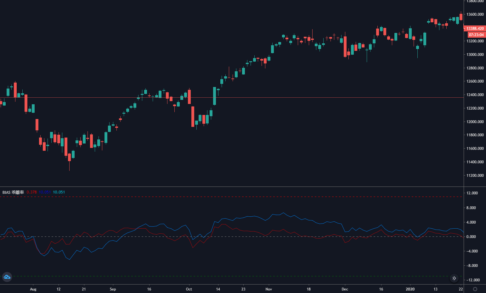
전략 논리
오차율은 이동평균의 또 다른 형태이기 때문에, 이중 이동평균 전략을 기반으로 하는 이중 오차율 전략을도 적용할 수 있다. 단기 오차율과 장기 오차율 사이의 위치 관계를 판단하면, 현재 시장 상태가 판단된다. 장기 오차율이 단기 오차율보다 크다면, 실제로는 단기 이동평균을 가로질러 상향으로 이동하는 단기 이동평균을 나타낸다.
- 긴 포지션 개설: 현재 보유 포지션이 없으며 장기 오차율이 단기 오차율보다 높으면
- 단기 포지션 개설: 현재 보유 포지션이 없으며 장기 오차율이 단기 오차율보다 낮으면
- 긴 포지션 폐쇄: 장기적인 오차율이 단기적인 오차율보다 낮고 장기적인 오차율이 단기적인 오차율보다 낮을 경우
- 단기 포지션 폐쇄: 단기 포지션 보유가 있고, 장기 오차율이 단기 오차율보다 크면
전략 작성
단계 1: 전략 프레임워크를 작성
# Strategy main function
def onTick():
     pass


# Program entry
def main():
     while True: # Enter infinite loop mode
         onTick() # execution strategy main function
         Sleep(1000) # sleep for 1 second
FMZ 플랫폼은 회전 훈련 모드를 채택합니다.main기능 및onTick함수 정의가 필요합니다. 주요 함수는 전략의 입력 함수이며, 프로그램은 주요 함수에서 시작하여 코드 라인씩 실행합니다. 주요 함수에서while루프를 반복해서 실행onTick전략의 모든 핵심 코드는onTick function.
단계 2: 가상 위치 정의
mp = 0
가상 포지션의 장점은 간단하게 작성되고 반복 작업이 빠르다는 것입니다. 일반적으로 백테스트 환경에서 사용됩니다. 모든 주문이 완전히 채워졌다고 가정하지만 실제 포지션은 일반적으로 실제 거래에서 사용됩니다. 가상 포지션은 개점 및 종료 후 상태를 기록하기 때문에 글로벌 변수로 정의되어야합니다.
단계 3: K 라인을 얻으십시오.
exchange.SetContractType('rb000') # Subscribe to futures varieties
bars_arr = exchange.GetRecords() # Get K-line array
if len(bars_arr) <long + 1: # If the number of K lines is too small
     return
FMZ 함수를 사용함SetContractType, 당신은 GetRecordsrebar 인덱스의 K-라인 데이터를 얻기 위한 함수입니다. 편차 비율을 계산하는 데 일정 기간이 걸리기 때문에, 프로그램 오류를 피하기 위해, 충분한 K 라인이 없다면, 사용if필터링하는 명령어
단계 4: 오차 비율을 계산합니다.
close = bars_arr[-2]['Close'] # Get the closing price of the previous K line
ma1 = TA.MA(bars_arr, short)[-2] # Calculate the short-term moving average value of the previous K line
bias1 = (close-ma1) / ma1 * 100 # Calculate the short-term deviation rate value
ma2 = TA.MA(bars_arr, long)[-2] # Calculate the long-term average of the previous K line
bias2 = (close-ma2) / ma2 * 100 # Calculate the long-term deviation rate value
오차율을 계산하는 공식에 따르면 먼저 폐쇄 가격을 얻습니다. 이 전략에서 우리는 이전 K 라인 폐쇄 가격을 사용합니다. 즉, 현재 K 라인 신호가 설정되고 다음 K 라인은 주문을하는 것입니다.talib예를 들어, 이동 평균은:TA.MA이 함수는 2개의 매개 변수를 받습니다. K선 배열과 이동 평균 기간입니다.
단계 5: 주문을 하는 것
global mp # global variables
current_price = bars_arr[-1]['Close'] # latest price
if mp> 0: # If you are holding long positions
    if bias2 <= bias1: # If the long-term deviation rate is less than or equal to the short-term deviation rate
        exchange.SetDirection("closebuy") # Set the trading direction and type
        exchange.Sell(current_price-1, 1) # Closing long positions
        mp = 0 # reset virtual holding positions
if mp <0: # If you are holding short positions
    if bias2 >= bias1: # If the long-term deviation rate is greater than or equal to the short-term deviation rate
        exchange.SetDirection("closesell") # Set the trading direction and type
        exchange.Buy(current_price + 1, 1) # closing short positions
        mp = 0 # reset virtual holding positions
if mp == 0: # If there is no holding position
    if bias2> bias1: # Long-term deviation rate is greater than short-term deviation rate
        exchange.SetDirection("buy") # Set the trading direction and type
        exchange.Buy(current_price + 1, 1) # open long positions
        mp = 1 # reset virtual holding position
    if bias2 <bias1: # The long-term deviation rate is less than the short-term deviation rate
        exchange.SetDirection("sell") # Set the trading direction and type
        exchange.Sell(current_price-1, 1) # open short positions
        mp = -1 # reset virtual holding position
전체 전략
# Backtest configuration
'''backtest
start: 2018-01-01 00:00:00
end: 2020-01-01 00:00:00
period: 1h
basePeriod: 1h
exchanges: [{"eid":"Futures_CTP","currency":"FUTURES"}]
'''

# External parameters
short = 10
long = 50


# Global variables
mp = 0


# Strategy main function
def onTick():
    # retrieve data
    exchange.SetContractType('rb000') # Subscribe to futures varieties
    bars_arr = exchange.GetRecords() # Get K-line array
    if len(bars_arr) <long + 1: # If the number of K lines is too small
        return

    # Calculate BIAS
    close = bars_arr[-2]['Close'] # Get the closing price of the previous K line
    ma1 = TA.MA(bars_arr, short)[-2] # Calculate the short-term moving average of the previous K line
    bias1 = (close-ma1) / ma1 * 100 # Calculate the short-term deviation rate value
    ma2 = TA.MA(bars_arr, long)[-2] # Calculate the long-term average of the previous K line
    bias2 = (close-ma2) / ma2 * 100 # Calculate the long-term deviation rate value

    # Placing Orders
    global mp # global variables
    current_price = bars_arr[-1]['Close'] # latest price
    if mp> 0: # If you are holding long positions
        if bias2 <= bias1: # If the long-term deviation rate is less than or equal to the short-term deviation rate
            exchange.SetDirection("closebuy") # Set the trading direction and type
            exchange.Sell(current_price-1, 1) # closing long positions
            mp = 0 # reset virtual holding position
    if mp <0: # If you are holding short positions
        if bias2 >= bias1: # If the long-term deviation rate is greater than or equal to the short-term deviation rate
            exchange.SetDirection("closesell") # Set the trading direction and type
            exchange.Buy(current_price + 1, 1) # closing short positions
            mp = 0 # reset virtual holding position
    if mp == 0: # If there is no holding position
        if bias2> bias1: # Long-term deviation rate is greater than short-term deviation rate
            exchange.SetDirection("buy") # Set the trading direction and type
            exchange.Buy(current_price + 1, 1) # opening long positions
            mp = 1 # reset virtual holding position
        if bias2 <bias1: # The long-term deviation rate is less than the short-term deviation rate
            exchange.SetDirection("sell") # Set the trading direction and type
            exchange.Sell(current_price-1, 1) # open short positions
            mp = -1 # reset virtual holding position


# Program entry function
def main():
    while True: # loop
        onTick() # execution strategy main function
        Sleep(1000) # sleep for 1 second
전체 전략은 FMZ 홈페이지에 공개되었습니다.https://www.fmz.com/strategy/215129
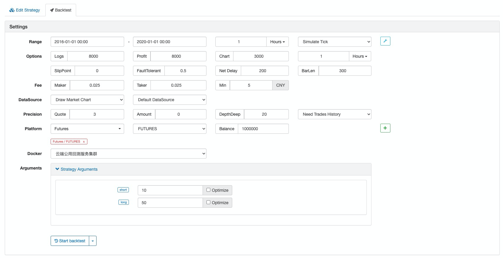
전략 백테스트
백테스트 구성
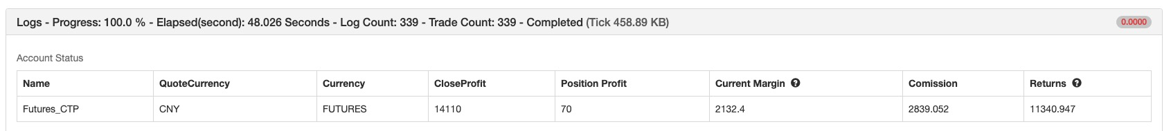
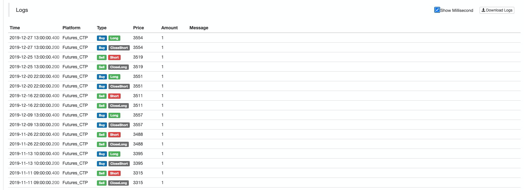
성과 보고
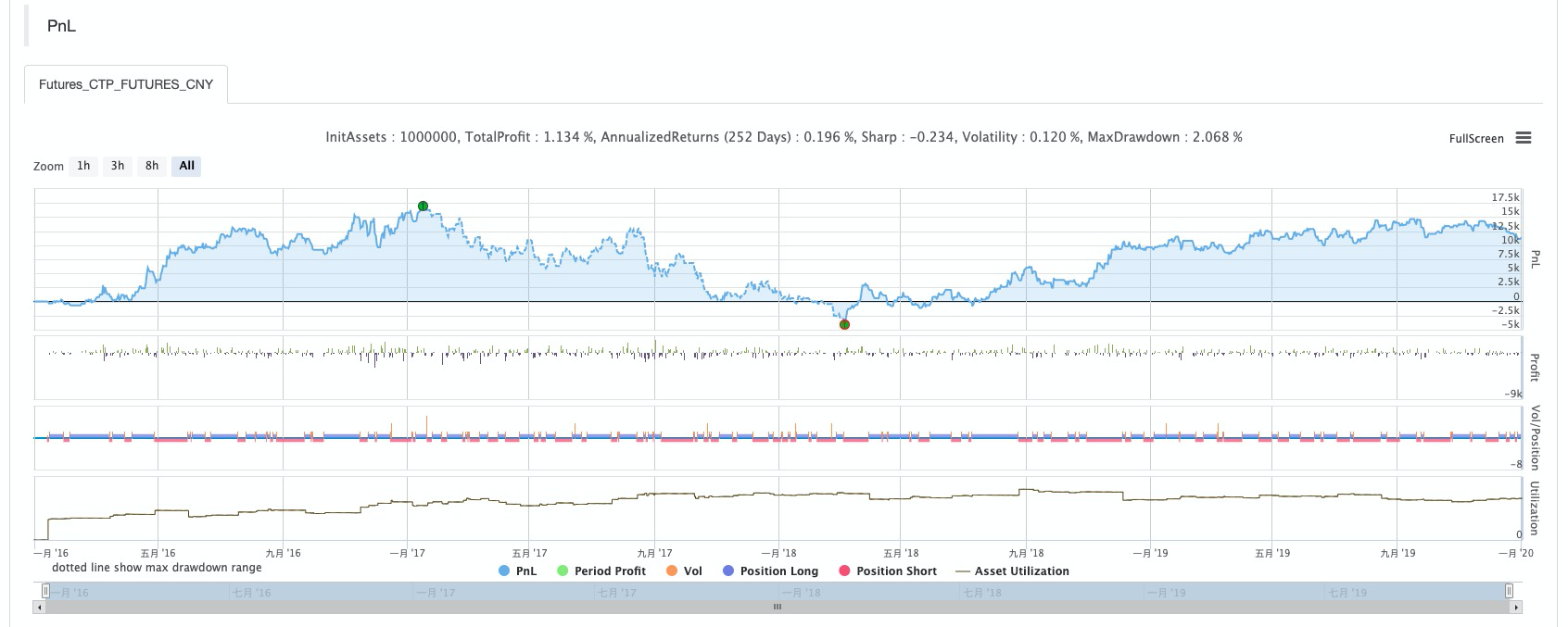
기금 곡선
요약
오차율은 트레이더에게 효과적인 참조를 제공할 수 있는 간단하고 효과적인 거래 도구입니다. 실제 사용에서는 MACD 및 볼링거 밴드 지표와 함께 유연하게 적용하여 그 가치를 진정으로 반영할 수 있습니다.
- 암호화폐 시장의 근본 분석을 정량화: 데이터를 스스로 이야기하도록!
- 동전圈의 기초적인 양적 연구 - 더 이상 모든
선생님들을 믿지 말고, 데이터를 객관적으로 이야기하십시오! - 양적 거래의 필수 도구 - 발명자 양적 데이터 탐색 모듈
- 모든 것을 마스터 - FMZ에 대한 소개 트레이딩 터미널의 새로운 버전 (TRB 중재 소스 코드)
- FMZ의 새로운 거래 단말기 소개 (TRB 리비트 소스 추가)
- FMZ 퀀트: 암호화폐 시장에서 공통 요구 사항 설계 예제 분석 (II)
- 80 줄의 코드에서 고주파 전략으로 뇌 없는 판매봇을 이용하는 방법
- FMZ 정량화: 암호화폐 시장의 일반적인 요구 디자인 사례 분석 (II)
- 80줄의 코드의 고주파 전략으로 뇌 없는 로봇을 파는 방법
- FMZ Quant: 암호화폐 시장에서 공통 요구 사항 디자인 예의 분석 (I)
- FMZ 정량화: 암호화폐 시장의 일반적인 요구 디자인 사례 분석 (1)