Внедрить стратегию количественной торговли цифровой валютой с двойным толчком в Python
Автор:Лидия., Создано: 2023-01-10 17:07:49, Обновлено: 2023-09-20 10:53:48
Внедрить стратегию количественной торговли цифровой валютой с двойным толчком в Python
Введение в алгоритм торговли Dual Thrust
Алгоритм двойной тяги - известная количественная стратегия торговли, разработанная Майклом Чалеком. Она обычно используется на фьючерсных, валютных и фондовых рынках.
В этой статье мы дадим подробные логические подробности этой стратегии и покажем, как реализовать этот алгоритм на платформе FMZ Quant. Прежде всего, нам нужно выбрать историческую цену предмета, с которым нужно торговать. Этот диапазон рассчитывается на основе цены закрытия, самой высокой цены и самой низкой цены за последние N дней. Когда рынок движется в определенном диапазоне от цены открытия, откройте позицию.
Мы протестировали эту стратегию с помощью одной торговой пары при двух общих рыночных условиях, а именно рынке тренда и рынке шока. Результаты показали, что система импульсной торговли лучше работает на рынке тренда и вызовет некоторые недействительные торговые сигналы на волатильном рынке. На рынке интервалов мы можем корректировать параметры для получения лучшей доходности. Для сравнения индивидуальных целевых торговых ориентиров мы также протестировали внутренний фьючерсный рынок товаров. Результат показал, что стратегия лучше средней производительности.
Принцип стратегии ДТ
Его логический прототип - это общая внутридневная стратегия торговли. Стратегия прорыва диапазона открытия основана на сегодняшней цене открытия плюс или минус определенный процент диапазона вчерашнего дня для определения верхнего и нижнего треков. Когда цена пересекает верхний трек, она откроет свою позицию для покупки, а когда она нарушит нижний трек, она откроет свою позицию для короткого.
Принцип стратегии
-
После закрытия вычисляются два значения: самая высокая цена - цена закрытия, и цена закрытия - самая низкая цена. Затем возьмем большую из двух значений и умножим значение на 0,7.
-
После того, как рынок открывается на следующий день, записывайте цену открытия и покупайте немедленно, когда цена превышает (цена открытия + стоимость запуска), или продавайте короткие позиции, когда цена ниже (цена открытия - стоимость запуска).
-
Эта стратегия не имеет очевидного стоп-лосса. Эта система является обратной системой, то есть, если есть ордер на короткую позицию, когда цена превышает (цену открытия + значение триггера), он отправит два ордера на покупку (один закрывает неправильную позицию, другой открывает правильную позицию). По той же причине, если цена длинной позиции ниже (цены открытия - значение триггера), он отправит два ордера на продажу.
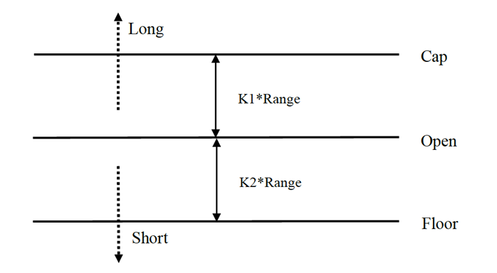
Математическое выражение стратегии ДТ
Диапазон = максимальный (HH-LC, HC-LL)
Метод расчета сигнала длинной позиции:
cap = открытый + K1 × Rangecap = открытый + K1 × Range
Метод расчета сигнала короткой позиции:
пол = открытый
Если K1 больше, чем K2, сигнал длинной позиции запускается, и наоборот. Для демонстрации мы выбираем K1=K2=0.5. В реальных сделках мы все еще можем использовать исторические данные для оптимизации этих параметров или корректировки параметров в соответствии с тенденциями рынка. Если вы быстрый, K1 должен быть меньше, чем K2. Если вы медвежий, K1 должен быть больше, чем K2.
Система является системой обратного движения. Поэтому, если инвесторы держат короткие позиции, когда цена пересекает верхний путь, они должны закрыть короткие позиции перед открытием длинных позиций. Если инвестор держит длинную позицию, когда цена переходит нижний путь, они должны закрыть длинную позицию перед открытием новой короткой позиции.
Улучшение стратегии ДТ:
При установке диапазона четыре ценовых точки (высокий, открытый, низкий и закрытый) предыдущих N дней вводятся, чтобы сделать диапазон относительно стабильным в определенный период, который можно применять к ежедневному отслеживанию тренда.
Условия запуска открытия длинных и коротких позиций стратегии, учитывая асимметричный диапазон, референтный диапазон длинных и коротких операций должен выбирать различное количество периодов, которые также могут определяться параметрами K1 и K2. Когда K1 < K2, сигнал длинной позиции относительно легко запускается, тогда как когда K1 > K2, сигнал короткой позиции относительно легко запускается.
Таким образом, при использовании этой стратегии, с одной стороны, вы можете ссылаться на лучшие параметры обратного тестирования исторических данных. С другой стороны, вы можете корректировать K1 и K2 поэтапно в соответствии с вашим суждением о будущем или других основных технических показателях периода.
Это типичный торговый метод ожидания сигналов, входа на рынок, арбитража, а затем выхода с рынка, но эффект превосходный.
Развернуть стратегию DT на платформе FMZ Quant
Мы открываем.FMZ.COM, войдите в аккаунт, нажмите на панель управления и разверните докер и робота.
Пожалуйста, ознакомьтесь с моей предыдущей статьей о том, как развернуть докер и робота:https://www.fmz.com/bbs-topic/9864.
Читатели, которые хотят приобрести собственный сервер облачных вычислений для развертывания докеров, могут обратиться к этой статье:https://www.fmz.com/digest-topic/5711.
Далее мы нажимаем на библиотеку стратегии в левом столбце и нажимаем на добавление стратегии.
Помните, чтобы выбрать язык программирования как Python в правом верхнем углу страницы редактирования стратегии, как показано на рисунке:
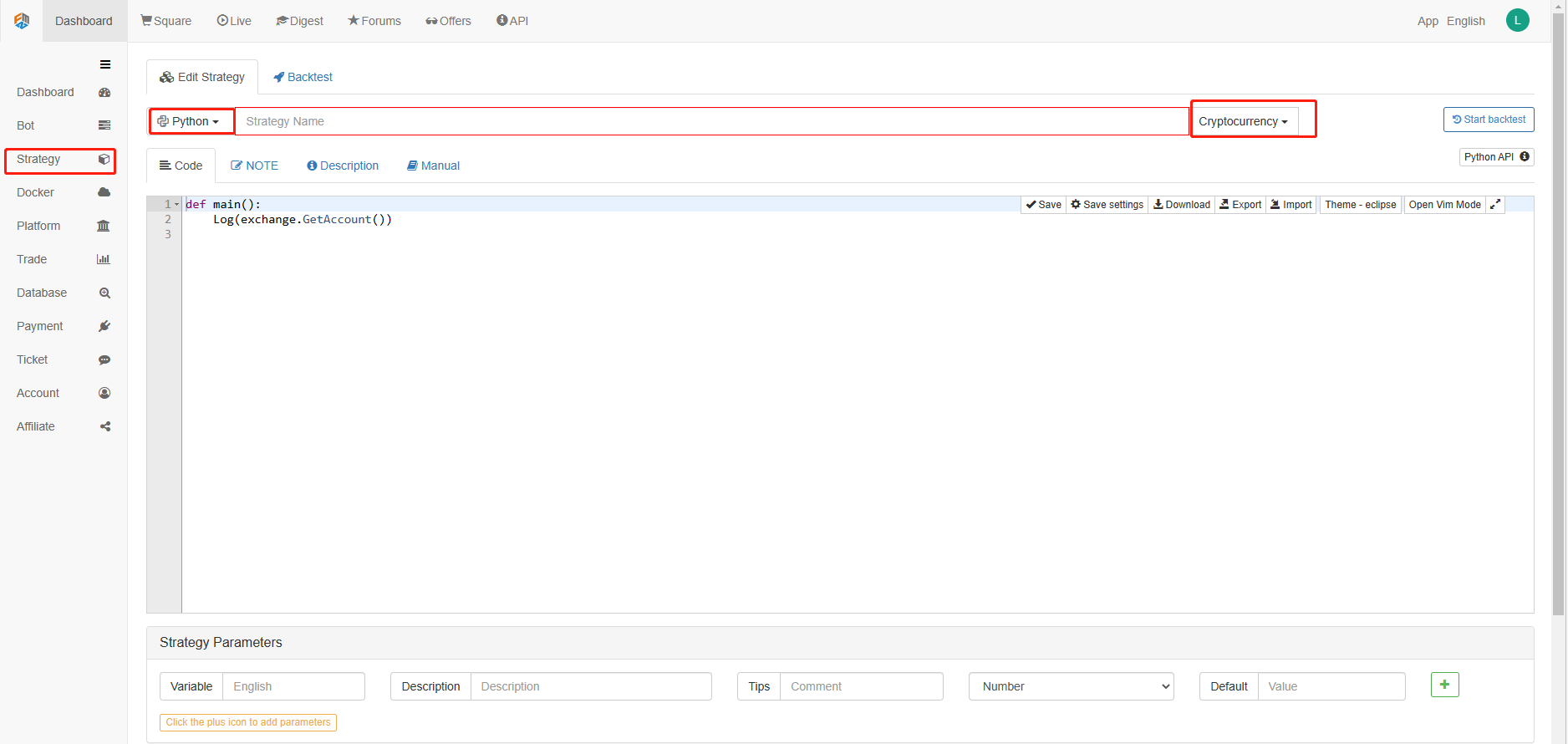
Далее мы напишем код Python на странице редактирования кода.
Мы будем использовать фьючерсы OKCoin для тестирования стратегии:
import time # Here we need to introduce the time library that comes with python, which will be used later in the program.

class Error_noSupport(BaseException): # We define a global class named ChartCfg to initialize the strategy chart settings. Object has many attributes about the chart function. Chart library: HighCharts.
    def __init__(self): # log out prompt messages
        Log("Support OKCoin Futures only! #FF0000")

class Error_AtBeginHasPosition(BaseException):
    def __init__(self):
        Log("Start with a futures position! #FF0000")

ChartCfg = {
    '__isStock': True, # This attribute is used to control whether to display a single control data series (you can cancel the display of a single data series on the chart). If you specify __isStock: false, it will be displayed as a normal chart.
    'title': { # title is the main title of the chart
        'text': 'Dual Thrust upper and bottom track chart' # An attribute of the title text is the text of the title, here set to 'Dual Thrust upper and bottom track chart' the text will be displayed in the title position.
    },
    'yAxis': { # Settings related to the Y-axis of the chart coordinate.
        'plotLines': [{ # Horizontal lines on the Y-axis (perpendicular to the Y-axis), the value of this attribute is an array, i.e. the setting of multiple horizontal lines.
            'value': 0, # Coordinate value of horizontal line on Y-axis
            'color': 'red', # Color of horizontal line
            'width': 2, # Line width of horizontal line
            'label': {  # Labels on the horizontal line
                'text': 'Upper track', # Text of the label
                'align': 'center' # The display position of the label, here set to center (i.e.: 'center')
            },
        }, {       # The second horizontal line ([{...} , {...}] the second element in the array)
            'value': 0, # Coordinate value of horizontal line on Y-axis
            'color': 'green', # Color of horizontal line
            'width': 2,  # Line width of horizontal line
            'label': { # Label
                'text': 'bottom track',
                'align': 'center'
            },
        }]
    },
    'series': [{ # Data series, that is, data used to display data lines, K-lines, tags, and other contents on the chart. It is also an array whose first index is 0.
        'type': 'candlestick', # Type of data series with index 0: 'candlestick' indicates a K-line chart.
        'name': 'Current period',  # Name of the data series
        'id': 'primary', # The ID of the data series, which is used for the related settings of the next data series.
        'data': []  # An array of data series to store specific K-line data
    }, {
        'type': 'flags',  # Data series, type: 'flags', display labels on the chart, indicating going long and going short. Index is 1.
        'onSeries': 'primary',  # This attribute indicates that the label is displayed on id 'primary'.
        'data': []    # The array that holds the label data.
    }]
}

STATE_IDLE = 0  # Status constants, indicating idle
STATE_LONG = 1 # Status constants, indicating long positions
STATE_SHORT = 2 # Status constants, indicating short positions
State = STATE_IDLE # Indicates the current program status, assigned as idle initially

LastBarTime = 0  # The time stamp of the last column of the K-line (in milliseconds, 1000 milliseconds is equal to 1 second, and the timestamp is the number of milliseconds from January 1, 1970 to the present time is a large positive integer).
UpTrack = 0   # Upper track value
BottomTrack = 0 # Bottom track value
chart = None # It is used to accept the chart control object returned by the Chart API function. Use this object (chart) to call its member function to write data to the chart.
InitAccount = None # Initial account status
LastAccount = None # Latest account status
Counter = { # Counters for recording profit and loss counts
    'w': 0, # Number of wins
    'l': 0  # Number of losses
}

def GetPosition(posType):  # Define a function to store account position information
    positions = exchange.GetPosition() # exchange.GetPosition() is the FMZ Quant official API. For its usage, please refer to the official API document: https://www.fmz.com/api.
    return [{'Price': position['Price'], 'Amount': position['Amount']} for position in positions if position['Type'] == posType] # Return to various position information

def CancelPendingOrders(): # Define a function specifically for withdrawing orders
    while True: # Loop check
        orders = exchange.GetOrders() # If there is a position
        [exchange.CancelOrder(order['Id']) for order in orders if not Sleep(500)] # Withdrawal statement
        if len(orders) == 0: # Logical judgment
            break

def Trade(currentState,nextState): # Define a function to determine the order placement logic.
    global InitAccount,LastAccount,OpenPrice,ClosePrice # Define the global scope
    ticker = _C(exchange.GetTicker) # For the usage of _C, please refer to: https://www.fmz.com/api.
    slidePrice = 1 # Define the slippage value
    pfn = exchange.Buy if nextState == STATE_LONG else exchange.Sell # Buying and selling judgment logic
    if currentState != STATE_IDLE: # Loop start
        Log(_C(exchange.GetPosition)) # Log information
        exchange.SetDirection("closebuy" if currentState == STATE_LONG else "closesell") # Adjust the order direction, especially after placing the order.
        while True:
            ID = pfn( (ticker['Last'] - slidePrice) if currentState == STATE_LONG else (ticker['Last'] + slidePrice), AmountOP) # Price limit order, ID=pfn (- 1, AmountOP) is the market price order, ID=pfn (AmountOP) is the market price order.
            Sleep(Interval) # Take a break to prevent the API from being accessed too often and your account being blocked.
            Log(exchange.GetOrder(ID)) # Log information
            ClosePrice = (exchange.GetOrder(ID))['AvgPrice'] # Set the closing price
            CancelPendingOrders() # Call the withdrawal function
            if len(GetPosition(PD_LONG if currentState == STATE_LONG else PD_SHORT)) == 0: # Order withdrawal logic
                break
        account = exchange.GetAccount() # Get account information
        if account['Stocks'] > LastAccount['Stocks']: # If the current account currency value is greater than the previous account currency value.
            Counter['w'] += 1 # In the profit and loss counter, add one to the number of profits.
        else:
            Counter['l'] += 1 # Otherwise, add one to the number of losses.
        Log(account) # log information
        LogProfit((account['Stocks'] - InitAccount['Stocks']),"Return rates:", ((account['Stocks'] - InitAccount['Stocks']) * 100 / InitAccount['Stocks']),'%')
        Cal(OpenPrice,ClosePrice)
        LastAccount = account

    exchange.SetDirection("buy" if nextState == STATE_LONG else "sell") # The logic of this part is the same as above and will not be elaborated.
    Log(_C(exchange.GetAccount))
    while True:
        ID = pfn( (ticker['Last'] + slidePrice) if nextState == STATE_LONG else (ticker['Last'] - slidePrice), AmountOP)
        Sleep(Interval)
        Log(exchange.GetOrder(ID))
        CancelPendingOrders()
        pos = GetPosition(PD_LONG if nextState == STATE_LONG else PD_SHORT)
        if len(pos) != 0:
            Log("Average price of positions",pos[0]['Price'],"Amount:",pos[0]['Amount'])
            OpenPrice = (exchange.GetOrder(ID))['AvgPrice']
            Log("now account:",exchange.GetAccount())
            break

def onTick(exchange): # The main function of the program, within which the main logic of the program is processed.
    global LastBarTime,chart,State,UpTrack,DownTrack,LastAccount # Define the global scope
    records = exchange.GetRecords() # For the usage of exchange.GetRecords(), please refer to: https://www.fmz.com/api.
    if not records or len(records) <= NPeriod: # Judgment statements to prevent accidents.
        return
    Bar = records[-1] # Take the penultimate element of records K-line data, that is, the last bar.
    if LastBarTime != Bar['Time']:
        HH = TA.Highest(records, NPeriod, 'High')  # Declare the HH variable, call the TA.Highest function to calculate the maximum value of the highest price in the current K-line data NPeriod period and assign it to HH.
        HC = TA.Highest(records, NPeriod, 'Close') # Declare the HC variable to get the maximum value of the closing price in the NPeriod period.
        LL = TA.Lowest(records, NPeriod, 'Low') # Declare the LL variable to get the minimum value of the lowest price in the NPeriod period.
        LC = TA.Lowest(records, NPeriod, 'Close') # Declare LC variable to get the minimum value of the closing price in the NPeriod period. For specific TA-related applications, please refer to the official API documentation.

        Range = max(HH - LC, HC - LL)  # Calculate the range
        UpTrack = _N(Bar['Open'] + (Ks * Range))  # The upper track value is calculated based on the upper track factor Ks of the interface parameters such as the opening price of the latest K-line bar.
        DownTrack = _N(Bar['Open'] - (Kx * Range)) # Calculate the down track value
        if LastBarTime > 0: # Because the value of LastBarTime initialization is set to 0, LastBarTime>0 must be false when running here for the first time. The code in the if block will not be executed, but the code in the else block will be executed.
            PreBar = records[-2] # Declare a variable means "the previous Bar" assigns the value of the penultimate Bar of the current K-line to it.
            chart.add(0, [PreBar['Time'], PreBar['Open'], PreBar['High'], PreBar['Low'], PreBar['Close']], -1) # Call the add function of the chart icon control class to update the K-line data (use the penultimate bar of the obtained K-line data to update the last bar of the icon, because a new K-line bar is generated).
        else:  # For the specific usage of the chart.add function, see the API documentation and the articles in the forum. When the program runs for the first time, it must execute the code in the else block. The main function is to add all the K-lines obtained for the first time to the chart at one time.
            for i in range(len(records) - min(len(records), NPeriod * 3), len(records)): # Here, a for loop is executed. The number of loops uses the minimum of the K-line length and 3 times the NPeriod, which can ensure that the initial K-line will not be drawn too much and too long. Indexes vary from large to small.
                b = records[i] # Declare a temporary variable b to retrieve the K-line bar data with the index of records.length - i for each loop.
                chart.add(0,[b['Time'], b['Open'], b['High'], b['Low'], b['Close']]) # Call the chart.add function to add a K-line bar to the chart. Note that if the last parameter of the add function is passed in -1, it will update the last Bar (column) on the chart. If no parameter is passed in, it will add Bar to the last. After executing the loop of i=2 (i-- already, now it's 1), it will trigger i > 1 for false to stop the loop. It can be seen that the code here only processes the bar of records.length - 2, and the last Bar is not processed.
        chart.add(0,[Bar['Time'], Bar['Open'], Bar['High'], Bar['Low'], Bar['Close']]) # Since the two branches of the above if do not process the bar of records.length - 1, it is processed here. Add the latest Bar to the chart.
        ChartCfg['yAxis']['plotLines'][0]['value'] = UpTrack  # Assign the calculated upper track value to the chart object (different from the chart control object chart) for later display.
        ChartCfg['yAxis']['plotLines'][1]['value'] = DownTrack # Assign lower track value
        ChartCfg['subtitle'] = { # Set subtitle
            'text': 'upper tarck' + str(UpTrack) + 'down track' + str(DownTrack) # Subtitle text setting. The upper and down track values are displayed on the subtitle.
        }
        chart.update(ChartCfg) # Update charts with chart class ChartCfg.
        chart.reset(PeriodShow) # Refresh the PeriodShow variable set according to the interface parameters, and only keep the K-line bar of the number of PeriodShow values.

        LastBarTime = Bar['Time'] # The timestamp of the newly generated Bar is updated to LastBarTime to determine whether the last Bar of the K-line data acquired in the next loop is a newly generated one.
    else: # If LastBarTime is equal to Bar.Time, that is, no new K-line Bar is generated. Then execute the code in {..}.
        chart.add(0,[Bar['Time'], Bar['Open'], Bar['High'], Bar['Low'], Bar['Close']], -1) # Update the last K-line bar on the chart with the last Bar of the current K-line data (the last Bar of the K-line, i.e. the Bar of the current period, is constantly changing).
    LogStatus("Price:", Bar["Close"], "up:", UpTrack, "down:", DownTrack, "wins:", Counter['w'], "losses:", Counter['l'], "Date:", time.time()) # The LogStatus function is called to display the data of the current strategy on the status bar.
    msg = "" # Define a variable msg.
    if State == STATE_IDLE or State == STATE_SHORT: # Judge whether the current state variable State is equal to idle or whether State is equal to short position. In the idle state, it can trigger long position, and in the short position state, it can trigger a long position to be closed and sell the opening position.
        if Bar['Close'] >= UpTrack: # If the closing price of the current K-line is greater than the upper track value, execute the code in the if block.
            msg = "Go long, trigger price:" + str(Bar['Close']) + "upper track" + str(UpTrack) # Assign a value to msg and combine the values to be displayed into a string.
            Log(msg) # message
            Trade(State, STATE_LONG) # Call the Trade function above to trade.
            State = STATE_LONG # Regardless of opening long positions or selling the opening position, the program status should be updated to hold long positions at the moment.
            chart.add(1,{'x': Bar['Time'], 'color': 'red', 'shape': 'flag', 'title': 'long', 'text': msg}) # Add a marker to the corresponding position of the K-line to show the open long position.

    if State == STATE_IDLE or State == STATE_LONG: # The short direction is the same as the above, and will not be repeated. The code is exactly the same.
        if Bar['Close'] <= DownTrack:
            msg = "Go short, trigger price:" + str(Bar['Close']) + "down track" + str(DownTrack)
            Log(msg)
            Trade(State, STATE_SHORT)
            State = STATE_SHORT
            chart.add(1,{'x': Bar['Time'], 'color': 'green', 'shape': 'circlepin', 'title': 'short', 'text': msg})

OpenPrice = 0 # Initialize OpenPrice and ClosePrice
ClosePrice = 0
def Cal(OpenPrice, ClosePrice): # Define a Cal function to calculate the profit and loss of the strategy after it has been run.
    global AmountOP,State
    if State == STATE_SHORT:
        Log(AmountOP,OpenPrice,ClosePrice,"Profit and loss of the strategy:", (AmountOP * 100) / ClosePrice - (AmountOP * 100) / OpenPrice, "Currencies, service charge:", - (100 * AmountOP * 0.0003), "USD, equivalent to:", _N( - 100 * AmountOP * 0.0003/OpenPrice,8), "Currencies")
        Log(((AmountOP * 100) / ClosePrice - (AmountOP * 100) / OpenPrice) + (- 100 * AmountOP * 0.0003/OpenPrice))
    if State == STATE_LONG:
        Log(AmountOP,OpenPrice,ClosePrice,"Profit and loss of the strategy:", (AmountOP * 100) / OpenPrice - (AmountOP * 100) / ClosePrice, "Currencies, service charge:", - (100 * AmountOP * 0.0003), "USD, equivalent to:", _N( - 100 * AmountOP * 0.0003/OpenPrice,8), "Currencies")
        Log(((AmountOP * 100) / OpenPrice - (AmountOP * 100) / ClosePrice) + (- 100 * AmountOP * 0.0003/OpenPrice))

def main(): # The main function of the strategy program. (entry function)
    global LoopInterval,chart,LastAccount,InitAccount # Define the global scope
    if exchange.GetName() != 'Futures_OKCoin':  # Judge if the name of the added exchange object (obtained by the exchange.GetName function) is not equal to 'Futures_OKCoin', that is, the object added is not OKCoin futures exchange object.
        raise Error_noSupport # Throw an exception
    exchange.SetRate(1) # Set various parameters of the exchange.
    exchange.SetContractType(["this_week","next_week","quarter"][ContractTypeIdx])  # Determine which specific contract to trade.
    exchange.SetMarginLevel([10,20][MarginLevelIdx]) # Set the margin rate, also known as leverage.

    if len(exchange.GetPosition()) > 0: # Set up fault tolerance mechanism.
        raise Error_AtBeginHasPosition
    CancelPendingOrders()
    InitAccount = LastAccount = exchange.GetAccount()
    LoopInterval = min(1,LoopInterval)
    Log("Trading platforms:",exchange.GetName(), InitAccount)
    LogStatus("Ready...")

    LogProfitReset()
    chart = Chart(ChartCfg)
    chart.reset()

    LoopInterval = max(LoopInterval, 1)
    while True: # Loop the whole transaction logic and call the onTick function.
        onTick(exchange)
        Sleep(LoopInterval * 1000) # Take a break to prevent the API from being accessed too frequently and the account from being blocked.
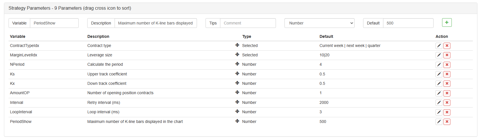
После написания кода, обратите внимание, что мы не закончили всю стратегию. Далее нам нужно добавить параметры, используемые в стратегии на странице редактирования стратегии. Способ добавления очень прост. Просто нажмите знак плюс внизу диалогового окна для написания стратегии, чтобы добавить один за другим.
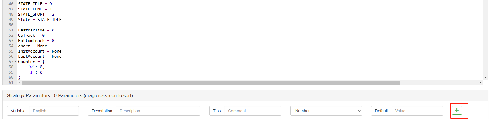
Содержание, которое необходимо добавить:
Пока что мы наконец-то закончили написание стратегии.
Обратное тестирование стратегии
После написания стратегии первое, что нам нужно сделать, это проверить ее на обратном пути, чтобы увидеть, как она ведет себя в исторических данных. Но обратите внимание, что результат бэкстеста не равен прогнозу будущего. Бэкстест может быть использован только в качестве ссылки для рассмотрения эффективности нашей стратегии. Как только рынок меняется, и стратегия начинает иметь большие потери, мы должны вовремя найти проблему, а затем изменить стратегию, чтобы адаптироваться к новой рыночной среде, такой как упомянутый порог. Если у стратегии есть потеря больше 10%, мы должны немедленно прекратить работу стратегии, а затем найти проблему. Мы можем начать с корректировки порога.
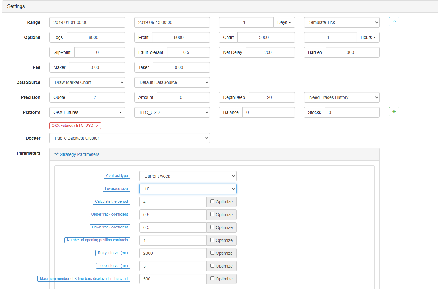
На странице редактирования стратегии нажмите на backtest. На странице backtest корректировка параметров может быть выполнена удобно и быстро в соответствии с различными потребностями. Особенно для стратегии со сложной логикой и многими параметрами, нет необходимости возвращаться к исходному коду и модифицировать его один за другим.
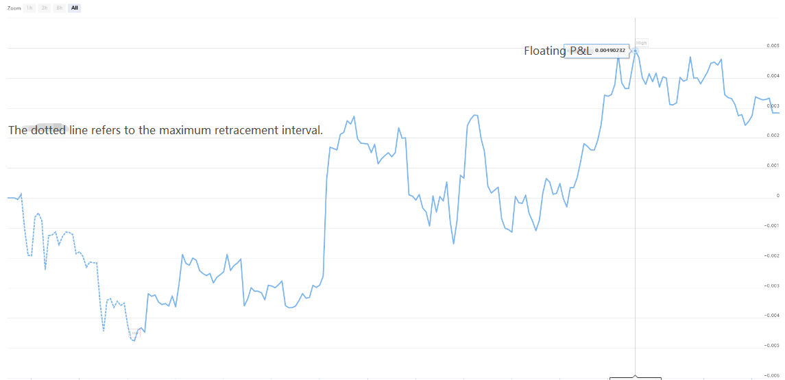
Время обратного тестирования - последние шесть месяцев.
Как видно, стратегия принесла хорошие результаты за последние полгода из-за очень хорошего одностороннего тренда BTC.

Если у вас есть какие-либо вопросы, вы можете оставить сообщение наhttps://www.fmz.com/bbs, будь то стратегия или технологии платформы, на платформе FMZ Quant есть профессионалы, готовые ответить на ваши вопросы.
- Количественный анализ фундаментального анализа на рынке криптовалют: пусть данные говорят сами за себя!
- Не стоит больше верить всяким хитроумным учителям, которые говорят, что данные объективны.
- Необходимый инструмент для количественной торговли - изобретатель модуля количественного исследования данных
- Освоение всего - Введение в FMZ Новая версия торгового терминала (с TRB Arbitrage Source Code)
- Ознакомьтесь с новым типом терминала FMZ (с кодом TRB)
- FMZ Quant: Анализ общих требований Примеры проектирования на рынке криптовалют (II)
- Как использовать бесмозговых роботов с высокочастотной стратегией в 80 строках кода
- Квалификация FMZ: Анализ примеров дизайна общих потребностей на рынке криптовалют (II)
- Как использовать высокочастотную стратегию 80-линейного кода для эксплуатации безмозговых роботов
- FMZ Quant: Анализ общих требований Примеры проектирования на рынке криптовалют (I)
- Квалификация FMZ: Анализ примеров дизайна общих потребностей на рынке криптовалют (1)