Machine learning compares the 8 major algorithms

Author: The Little Dream, Created: 2016-12-05 10:42:02, Updated:

Machine learning compares the 8 major algorithms

This article mainly reviews the adaptation scenarios of the following commonly used algorithms and their advantages and disadvantages!

There are so many machine learning algorithms in the field of classification, regression, grouping, recommendation, image recognition, etc. It is not easy to find a suitable algorithm, so in practical applications we generally experiment with inspirational learning.

Usually we start with the most commonly accepted algorithms, such as SVM, GBDT, Adaboost, which are now very popular in deep learning, and neural networks are also a good choice.

If you care about accuracy, the best approach is to test each algorithm individually through cross-validation, compare them, and then adjust the parameters to ensure that each algorithm achieves the optimal, and finally choose the best one.

But if you're just looking for an algorithm that's good enough to solve your problem, or here are some tips to use, we'll analyze the pros and cons of each algorithm below and make it easier to choose one based on the pros and cons of each algorithm.

Divergence and bias

In statistics, a model is good or bad, and it's measured in terms of bias and variance, so let's popularize bias and variance first:

Deviation: describes the difference between the expected E of the predicted value (the estimated value) and the actual value Y. The greater the deviation, the more the deviation from the actual data.

Difference: describes the range of variation of the predicted value P, the degree of discretion, the difference of the predicted value, the distance from its expected value E. The larger the difference, the more scattered the distribution of the data.

The true error of the model is the sum of the two, as shown in the figure below:

If it is a small training set, a classifier with a high/low bias (e.g., the naive Bayesian NB) has a greater advantage than a classifier with a low/high bias (e.g., the KNN) because the latter is over-fitted.

However, as your training set grows, the better the model is able to predict the original data, the less the bias, and the less the low-divergence/high-divergence classifiers gradually show their advantages (because they have lower approximation errors), the more the high-divergence classifiers are no longer sufficient to provide accurate models.

Of course, you can also think of this as a difference between the generation model (NB) and the determination model (KNN).

Why is it that simple Bayes is high-deviation low-deviation?

The following content is self-published:

First, suppose you know the relationship between the training set and the test set. In simple terms, we are going to learn a model on the training set and then get the test set to use, and the results will be measured based on the error rate of the test set.

But a lot of times, we can only assume that the test set and the training set match the same data distribution, but we don't get the real test data.

Since the training sample is small (at least not large enough), the model obtained through the training set is not always truly correct. Even if the training set is 100% correct, it does not mean that it maps the true data distribution.

Also, in practice, training samples often have some noise error, so if too much perfection is pursued on the training set, a very complex model can cause the model to treat the errors in the training set as true data distribution features, resulting in incorrect data distribution estimates.

In this way, the real test set is completely wrong (this phenomenon is called fit); but you can't use a model that is too simple, otherwise the model will not be enough to map the data distribution when the data distribution is relatively complex (which reflects a high error rate even on the training set, this phenomenon is less fit).

Overfitting indicates that the model used is more complex than the real data distribution, while underfitting indicates that the model used is simpler than the real data distribution.

In the context of statistical learning, when people sketch the model complexity, there is a view that Error = Bias + Variance. The error here can probably be understood as the model's prediction error rate, which is composed of two parts, one part is the estimate bias caused by the model being too simple, and the other part is the greater variation space and uncertainty caused by the model being too complex.

Thus, it is easy to analyze a simple Bayesian. It simply assumes that the data are unrelated and is a severely simplified model. So, for such a simple model, most cases will have a Bias part greater than the Variance part, i.e. high and low biases.

In practice, in order to keep the error as small as possible, we need to balance the ratio of Bias and Variance when selecting the model, i.e. balance over-fitting and under-fitting.

The relationship between deviation and variance and model complexity is made clearer using the following diagram:

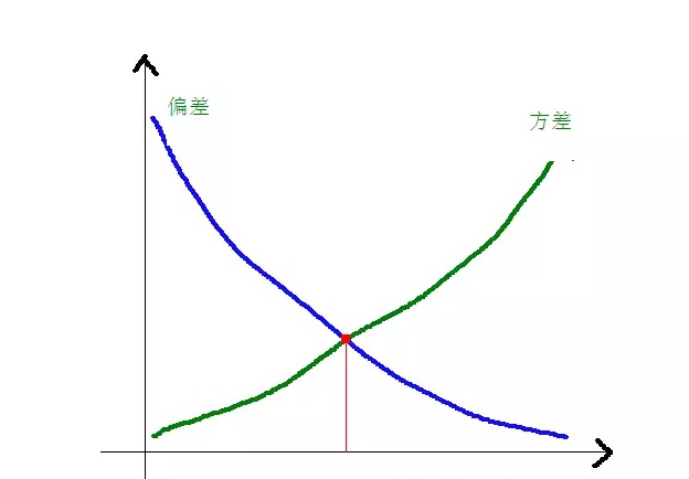
As the model complexity increases, the deviation gradually decreases, while the bias gradually increases.

Common advantages and disadvantages of algorithms
- 1.朴素贝叶斯
  
  Simple Bayes belongs to the generative model (about generative models and deterministic models, mainly on whether or not it requires a unified distribution), very simple, you just do a bunch of counting.
  
  If the conditional independence hypothesis (a more rigorous condition) is given, the convergence rate of a simple Bayesian classifier will be faster than that of a discrete model, such as a logical regression, so you only need less training data. Even if the NB conditional independence hypothesis does not hold, the NB classifier still performs very well in practice.
  
  Its main disadvantage is that it can't learn interactions between features, which in mRMR is called feature redundancy. To cite a more classic example, for example, although you like the films of Brad Pitt and Tom Cruise, it can't learn the films you don't like them in.
  
  Pros:
  
  The simplistic Bayesian model is derived from classical mathematical theory, with a solid mathematical foundation and stable classification efficiency. It performs well on small data, can handle multi-class tasks individually, and is suitable for incremental training. The algorithm is less sensitive to missing data and is simpler, often used for text classification. The disadvantages:
  
  It is necessary to calculate the prior probability. There is an error rate in classifying decisions. It is sensitive to the form of expression of the input data.
- 2.逻辑回归
  
  There are many ways to normalize models (L0, L1, L2, etc.) and you don't have to worry about whether your characteristics are related, as you would with a simple Bayesian.
  
  You also get a good probability explanation compared to decision trees and SVMs, and you can even easily use new data to update the model (using online gradient descent algorithms).
  
  If you need a probability architecture (e.g., to simply adjust the classification threshold, indicate uncertainty, or obtain confidence intervals), or you want to quickly integrate more training data into the model later, use it.
  
  Sigmoid function:
  
  Pros: To achieve a simple and widely applicable industrial problem; Very small computing volume, fast speeds, low storage resources; A convenient observation sample probability score; For logical regression, multilinearity is not a problem, it can be solved with L2 normalisation; The disadvantages: When character spaces are large, the performance of logical regression is not good; Easy to misfit, generally not very accurate Can't handle a large number of multiclass features or variables well It can only handle two classification problems (the derived softmax on this basis can be used for multi-classes) and must be linearly divisible; For non-linear features, conversion is required;
- 3.线性回归
  
  Linear regression is used for regression, unlike logistic regression for classification, and its basic idea is to optimize the error function of the least squares form using gradient descent.
  
  In LWLR (Local weighted linear regression), the computational expression of the parameters is:
  
  Thus, unlike LWLR, LWLR is a non-parametric model, as the training sample is traversed at least once each time a regression is performed.
  
  Pros: Simple to implement, easy to compute;
  
  Disadvantages: Not able to fit nonlinear data.
- 4.最近邻算法——KNN
  
  KNN stands for Nearest Neighbor Algorithm and its main processes are:
  1. Calculate the distance between each sample point in the training sample and the test sample (common distance measurements include European distance, Martian distance, etc.);
  2. All of the above distance values are sorted;
  3. Select the sample with the smallest distance k;
  4. The final classification category is determined by voting on the label of this sample k.
  How to choose an optimal K-value depends on the data. Generally, a higher K-value at classification can reduce the impact of noise, but blurs the lines between categories.
  
  A better K-value can be obtained through various inspirational techniques, such as cross-validation. The presence of additional noise and non-correlation feature vectors reduces the accuracy of the K-neighboring algorithm.
  
  Neighboring algorithms have stronger consistency results. As the data tends to infinity, the algorithm guarantees an error rate that does not exceed twice that of the Bayesian algorithm. For some good values of K, the K-neighboring algorithm guarantees an error rate that does not exceed the Bayesian theoretical error rate.
  
  The advantages of the KNN algorithm
  
  The theory is mature, the idea is simple, it can be used for both classification and regression. Can be used for non-linear classification; The training time complexity is O ((n); There are no assumptions about the data, high accuracy, and no sensitivity to outliers. Disadvantages
  
  It's a lot of computing. Sample imbalance problem (i.e. some categories have a large number of samples, while others have a small number of samples); It requires a lot of memory.
- 5.决策树
  
  Easy to explain. It can handle interactions between features without stress and is non-parametric, so you don't have to worry about anomalous values or whether the data is linearly separable (for example, a decision tree can easily handle category A at the end of a feature dimension x, category B in the middle, and then category A appears again at the front end of the feature dimension x).
  
  One of its disadvantages is that it does not support online learning, so the decision tree needs to be completely rebuilt after the new sample arrives.
  
  Another disadvantage is the ease with which over-fitting occurs, but this is also the entry point for integration approaches such as random forest RF (or tree boosted tree).
  
  In addition, random forest is often the winner of many classification problems (usually just a little bit better than support vectoring), it trains quickly and is adjustable, and you don't have to worry about tuning a bunch of parameters like support vectoring, so it has been popular in the past.
  
  It is important in decision trees to choose an attribute for branching, so pay attention to the calculation of the information gain formula and understand it in depth.
  
  The calculation formula for the information bar is as follows:
  
  where n represents n categorical categories (e.g. assuming 2 problems, then n=2) ‒ calculate the probabilities of p1 and p2 for these two types of samples in the total sample, respectively, so that the information bar before the unselected attribute branch can be calculated.
  
  Now that a property xixi is selected for branching, the branching rule is: if xi = vxi = v, divide the sample into one branch of the tree; if not equal, move to another branch.
  
  Obviously, the sample in the branch is likely to contain 2 categories, calculating the branches H1 and H2 respectively, and calculating the total information H1 = p1 H1 + p2 H2 after the branch, then the information gain ΔH = H - H. Using the principle of information gain, test all the attributes aside and select the one that gives the greatest gain as the attribute of this branch.
  
  The Benefits of Decision Trees
  
  The calculation is simple, easy to understand and explainable. A sample that is better suited to treatment with missing properties; It can handle unrelated features. This allows us to produce viable and effective results on large data sources in a relatively short time. Disadvantages
  
  In addition to the above, there are also a number of other types of forest that are likely to be over-adapted. The data is not relevant to each other. For data with inconsistent sample sizes across categories, information gain results in a decision tree that is biased towards features with more numerical values (which have this disadvantage as long as information gain is used, such as RF).
- 5.1 Adaboosting
  
  Adaboost is an additive model where each model is built on the basis of the error rate of the previous model, with an over-focus on the error-dividing sample and less focus on the correctly classified sample, which after iteration gives a relatively better model.
  
  Benefits
  
  Adaboost is a highly accurate classifier. Sub-classifiers can be built using various methods. Adaboost algorithm provides a framework. When using a simple classifier, the results calculated are understandable, and the construction of a weak classifier is extremely simple. It's simple, no feature filtering needed. It is not easy to overfitting. For combinatorial algorithms such as Random Forest and GBDT, refer to this article: Machine Learning - Summary of combinatorial algorithms
  
  Disadvantages: more sensitive to outliers
- 6.SVM支持向量机
  
  The high accuracy provides good theoretical assurance for avoiding over-fitting, and even if the data is linearly indivisible in the original character space, it works well as long as it is given a suitable core function.
  
  It is particularly popular in dynamic ultra-high-dimensional text classification problems. Unfortunately, memory consumption is high, it is difficult to explain, and running and tweaking are also a bit of a hassle, while random forest just avoids these disadvantages, which is more practical.
  
  Benefits It can solve high-dimensional problems, i.e. large feature spaces. It can handle interactions of nonlinear features. It is not necessary to rely on all the data. It can improve the ability to generalize.
  
  Disadvantages When the sample is large, it is not very efficient; when it is small, it is not very efficient. There is no universal solution to nonlinear problems, and it is sometimes difficult to find a suitable kernel function. It is sensitive to missing data. The choice of kernel is also a tricky one (libsvm comes with four kernel functions: linear kernel, polynomial kernel, RBF and sigmoid kernel):
  
  First, if the number of samples is less than the characteristic number, then it is not necessary to select a nonlinear nucleus, a simple linear nucleus can be used;
  
  Second, if the number of samples is greater than the number of features, then using nonlinear cores to map the sample to higher dimensions can generally yield better results.
  
  Third, if the number of samples and the number of traits are equal, the case can be used for nonlinear nuclei, the same principle as for the second type.
  
  For the first case, the data can also be dimensioned first, and then the nonlinear kernel is used, which is also a method.
- The advantages and disadvantages of artificial neural networks 7.
  
  The advantages of artificial neural networks: High accuracy of classification; It has strong parallel distributed processing, distributed storage and learning capabilities. It has strong robustness and fault tolerance for noise neurons, which can be used to approximate complex nonlinear relationships. It has a function of memory recall.
  
  The disadvantages of artificial neural networks: Neural networks require a large number of parameters, such as the initial value of the network topology structure, weight and threshold values. The inability to observe the learning process, the difficulty of interpreting the output, which can affect the credibility and acceptability of the results; The study time is too long and may not even reach the purpose of the study.
- 8 K-Means clusters
  
  I have written a previous article on K-Means clustering, link: Machine Learning Algorithms - K-Means Clustering.
  
  Benefits The algorithm is simple and easy to implement; For processing large data sets, the algorithm is relatively scalable and efficient because its complexity is about O ((nkt), where n is the number of all objects, k is the number of vertices, and t is the number of iterations. The algorithm tries to find the k partitions that make the square error function value the smallest. Clustering is better when the array is dense, spherical, or conical, and there is a clear distinction between arrays and arrays.
  
  Disadvantages High data type requirements for numerical data; It may converge to local minima, but it converges more slowly on large data. The K-value is more difficult to choose; Sensitive to the initial value of the centroid, which may lead to different clustering results for different initial values; It is not suitable for detecting non-convex shapes or for detecting large differences in size. A small amount of this data can have a significant impact on the mean value, which is sensitive to noise and isolated point data.
  
  Algorithm selects references
  
  In a previous article translated from abroad, one of them gave a simple algorithmic selection trick:
  
  The first thing that should be chosen is logical regression, and if its effect is not good, then its results can be used as a benchmark to compare with other algorithms on the basis;
  
  Then try a decision tree (random forest) to see if it can significantly improve your model's performance. Even if you don't end up using it as your final model, you can use a random forest to remove noise variables and make feature selections.
  
  If the number of features and observed samples is particularly large, then using an SVM is an option when resources and time are sufficient (this premise is important).
  
  Usually: GBDT>=SVM>=RF>=Adaboost>=Other... Well, deep learning is very popular now, it is used in many fields, it is based on neural networks, I am currently learning myself, but theoretical knowledge is not very thick, understanding is not deep enough, so I will not do an introduction here.
  
  Algorithms are important, but good data is better than good algorithms, and designing good features is very helpful. If you have a super-large data set, it may not have much impact on the classification performance regardless of which algorithm you use (when you can make choices based on speed and ease of use).
References