Sharp is 0.6, should we throw it out?

Sharp is 0.6, should we throw it out?

We did an experiment to illustrate this problem. This experiment started with some key assumptions. We had 20 trading signals with compound annual returns of 8% and an annualized Sharpe ratio of 0.6. This strategy signal was not very productive. These trading signals were issued every day.

• An important input variable in trading is the correlation between signals. We conducted a series of experiments according to correlation coefficients from 0 to 0.9. The experiments did not consider transaction costs (because we were only interested in relative performance) and the distribution of annualised portfolio returns, which were rebalanced daily according to correlation, was basically the same. Obviously, without considering strategic correlation, more than one strategy would not increase annualised returns.

  

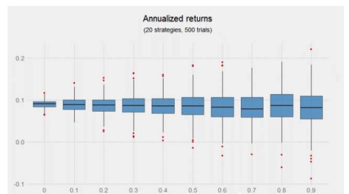
  Combining signals of low relevance together does not increase returns, but the diagram above suggests the potential benefits of increasing strategies, especially when these strategies are unrelated. The left half of the graph, the correlation coefficients from 0 to 0.4, has a narrower distribution and returns for five hundred experiments are positive.

  The results were clearer when the Sharpe ratio was used to measure risk-adjusted returns. A combination of 20 annualised Sharpe ratios of 0.6 and 0 with an annualised Sharpe ratio of 3 and 20 annualised Sharpe ratios of 0.6 and 0.9 with an average annualised Sharpe ratio of 0.64 yielded 370% higher returns.

  

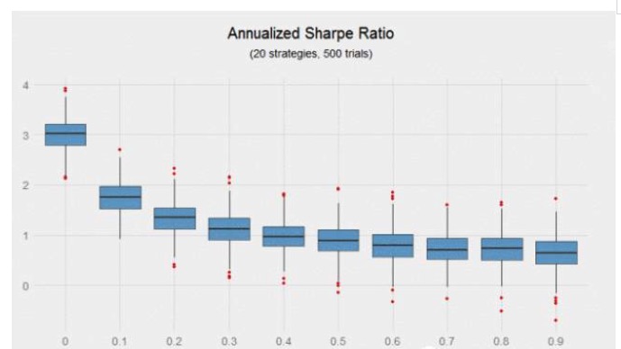
  It is noteworthy in the above graph that the Sharpe ratio decreases rapidly as the relevance of the strategy increases. The correlation coefficient increases from 0 to 0.2, and the Sharpe ratio decreases by 56%.

  Even with a very high Sharpe ratio, the combination strategy has nearly 50,000 trading signals, and the difference in Sharpe ratio of a zero-correlation combination is still surprising. A lucky investor may get a 3.5 Sharpe ratio (which may make a person a billionaire) while an unlucky investor with the same combination gets only a 2.5 Sharpe ratio. Even with a high Sharpe ratio combination, gas plays an important role.

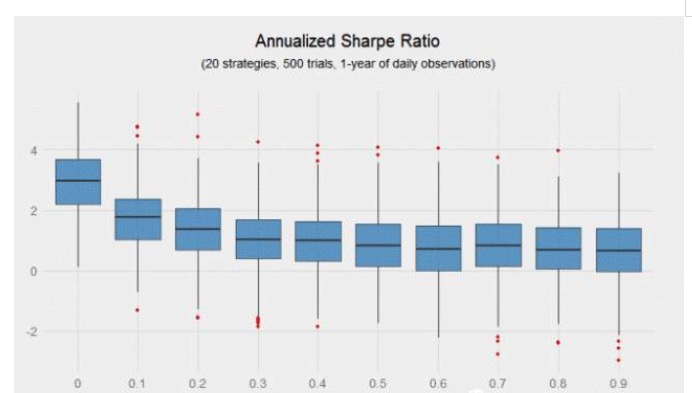
  Obviously, the more observational samples, the clearer the boundaries. What happens if an investor has only one year of observational samples instead of ten? The chart below shows that as correlation increases, the difference in the Sharpe ratio increases exponentially) Despite 5,000 trades, most portfolios cannot separate from the random luck component. Obviously, this is why data-driven hedge funds prefer high-frequency trading, where high-frequency trades can verify signals faster and achieve their average Sharpe ratio.

  

  If we simulate 10,000 of the above individual strategies, how many have a p-test value of less than 5%? The answer is close to 48%, which may lead most researchers to abandon such a routine strategy (i.e. the annualized Sharpe ratio of 0.6 strategy); however, if the correlation between signals is low enough that the combination of these weak signals can produce miracles, the return of the combination becomes very significant.

  

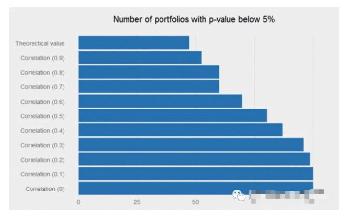
  A strategy with an annualized Sharpe ratio of 0.6 may be abandoned by researchers because it has no attraction in trading; but if it has the correct (i.e. low) correlation between the existing signals, then it can well add value to the portfolio.

  This article does not open up new areas, as the benefits of diversified investing are well known in the investment community. However, it does remind you that you do not need to abandon the 0.6 annualized Sharpe ratio strategy, perhaps you can add it to your existing strategy portfolio, thus reducing the liquidity of the portfolio and allowing more leverage to be used to improve overall returns.

Translated from private workshop