This article was inspired by my observations of some common warnings and pitfalls when attempting to apply machine learning techniques to trading problems while researching data on inventor quantification platforms.

If you haven't read my previous article, we recommend that you read my previous guide to automated data research environments and systematic methods for developing trading strategies built on the inventor quantification platform.

The address is here:https://www.fmz.com/digest-topic/4187andhttps://www.fmz.com/digest-topic/4169 这两篇文章.

How to Build a Research Environment

This tutorial is designed for amateurs, engineers, and data scientists of all skill levels, whether you are a bigwig or a novice programmer. The only skills you need are a basic understanding of the Python programming language and enough command-line operations to set up a data science project.

• Install inventor quantified hosts and set up Anaconda

发明者量化平台FMZ.COM除了提供优质的各大主流交易所的数据源，还提供一套丰富的API接口以帮助我们在完成数据的分析后进行自动化交易。这套接口包括查询账户信息，查询各个主流交易所的高，开，低，收价格，成交量，各种常用技术分析指标等实用工具，特别是对于实际交易过程中连接各大主流交易所的公共API接口，提供了强大的技术支持。

All of the above features are packaged into a Docker-like system, and all we have to do is buy or lease our own cloud computing service and then deploy the Docker system.

In the official name of the inventor's quantification platform, this Docker system is called the host system.

For more information on how to deploy hosts and bots, please refer to my previous post:https://www.fmz.com/bbs-topic/4140

Readers who want to buy their own cloud server deployment host can refer to this article:https://www.fmz.com/bbs-topic/2848

After successfully deploying a good cloud service and host system, next we'll install Python's biggest temple to date: Anaconda.

The easiest way to implement all the relevant programming environments (dependencies, version management, etc.) is to use Anaconda. It is a packed Python data science ecosystem and dependency library manager.

Since we are installing Anaconda on a cloud service, we recommend that the cloud server installs the command-line version of Anaconda on the Linux system.

For instructions on how to install Anaconda, please see the official guide to Anaconda:https://www.anaconda.com/distribution/

If you're an experienced Python programmer and don't feel the need to use Anaconda, that's totally fine. I'll assume you don't need help installing the necessary dependencies, you can skip this section.

Developing a trading strategy

The final output of the trading strategy should answer the following questions:

• Direction: Determine whether the asset is cheap, expensive or fair in value.

• 开仓条件：如果资产价格便宜或者昂贵，你应该做多或者做空.

• If the price of the asset is reasonable and we hold a position in the asset (previous purchase or sale), should you strike?

• Price range: the price (or range) at which the open position is traded

• Quantity: The amount of funds traded (e.g. number of digital currencies or number of hands on commodity futures)

Machine learning can be used to answer each of the above questions, but for the rest of this article, we will focus on answering the first question, which is trading direction.

Strategic approaches

There are two types of approaches to building strategies, one model-based and the other data-based mining; the two are essentially opposite approaches.

In model-based strategy building, we start with the market inefficiency model, which constructs mathematical expressions (e.g. price, yield) and tests their effectiveness over longer time cycles. The model is usually a simplified version of a truly complex model that needs to be validated for its meaning and stability over long cycles.

On the other hand, we first look for price patterns and try to use algorithms in data mining methods. The reasons for these patterns are not important because only certain patterns will continue to repeat in the future. This is a blind analysis method that requires rigorous testing to identify true patterns from random patterns.

Obviously, machine learning is easy to apply to data mining methods. Let's see how to use machine learning to create trading signals from data mining.

Code examples use inventor-based quantification platform retrieval tools and automated transaction API interfaces. After deploying the host and installing Anaconda in the above section, you just need to install the data science analytics library we need and the famous machine learning model scikit-learn.

pip install -U scikit-learn

Using machine learning to create trading strategy signals

• Data mining

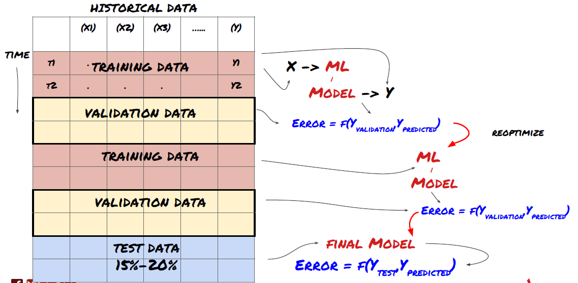
Before we get started, a standard machine learning problem system is shown in the diagram below:

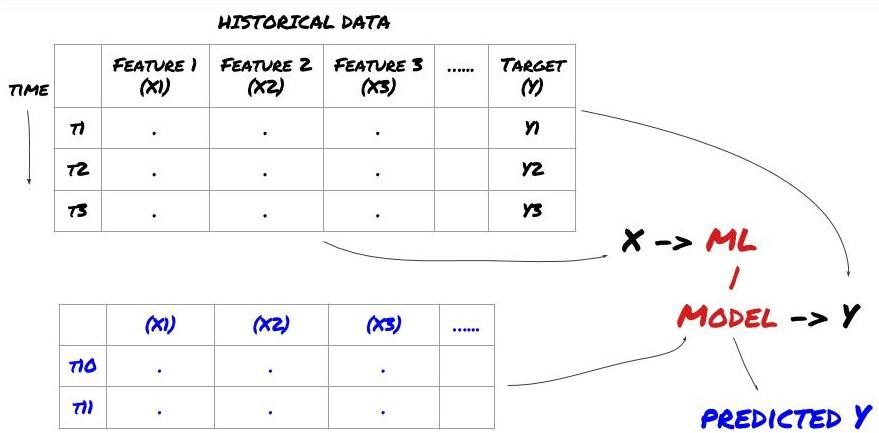
Machine learning problem system

The feature we're going to create must have some predictive capability ((X), we want to predict the target variable ((Y), and use historical data to train an ML model that can predict Y as close to the actual value as possible. Finally, we use this model to predict new data about Y that we don't know. This leads us to step one:

Step 1: Set your problems

• What do you want to predict? What's a good prediction? How do you rate the outcome of a prediction?

I mean, in our frame above, what is Y?

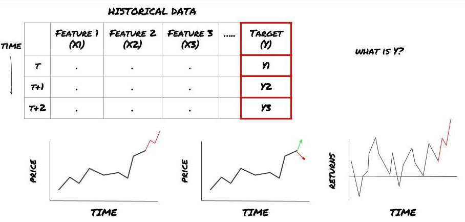
What do you want to predict?

Do you want to predict future prices, future returns/PNL, buy/sell signals, optimize portfolio allocation and try to execute trades efficiently etc?

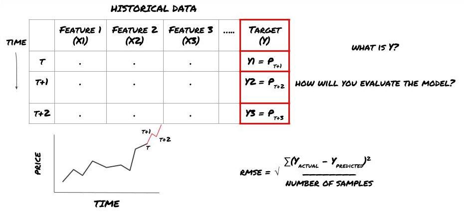
Suppose we try to predict the price on the next time frame. In this case, Y ((t) = price ((t + 1)). Now we can complete our framework with the historical data.

Note that Y (t) is known only in retrospect, but when we use our model we will not know the price at time t (t + 1) ‒ we use our model to predict Y (t) and only compare it to the actual value at time t + 1; this means that you cannot use Y as a feature in the prediction model.

Once we know the target Y, we can also decide how to evaluate our predictions. This is very important for distinguishing between different models of the data we will be trying. Depending on the problem we are solving, select an indicator that measures the efficiency of our model. For example, if we are predicting prices, we can use the equine root error as an indicator. Some common indicators (average, MACD and differential, etc.) are already pre-coded in the inventor's quantized toolkit, and you can call these indicators globally via an API interface.

ML framework used to predict future prices

To demonstrate this, we will create a predictive model to predict the future expected benchmark value of a hypothetical investment benchmark, where:

basis = Price of Stock — Price of Future

basis(t)=S(t)−F(t)

Y(t) = future expected value of basis = Average(basis(t+1),basis(t+2),basis(t+3),basis(t+4),basis(t+5))

Since this is a regression problem, we will evaluate the model on RMSE (square root error); we will also use Total Pnl as an evaluation criterion.

Note: For mathematical knowledge about RMSE, please refer to the related content of the encyclopedia

• 我们的目标：创建一个模型，使预测值尽可能接近Y.

Step two: Gather reliable data

Collect and clean up data that can help you solve the problem at hand

If we are predicting prices, you can use the price data of the investment indicator, the trading volume data of the investment indicator, similar data of the relevant investment indicator, the index of the investment indicator parity overall market indicator, the price of other relevant assets, etc.

You need to set up data access permissions for this data, and ensure that your data is accurate and correct, and address missing data (a very common problem); while ensuring that your data is unbiased and fully represents all market conditions (e.g., the same number of W/L scenarios) to avoid deviations in the model. You may also need to clean up the data to get dividends, split investment indices, continuity, etc.

If you are using the inventor's quantification platformFMZ.COMThe inventor quantification platform also pre-clears and filters this data, such as the breakdown of indices and deep market data, and presents it to the strategy developer in a format that is easy to understand by the quantification worker.

To facilitate the presentation, we use the following data as the Auquan MQK toolkit for virtual investment indicators, and we also talk about a very convenient quantification tool called Auquan's Toolbox, for more information, see:https://github.com/Auquan/auquan-toolbox-python

# Load the data
from backtester.dataSource.quant_quest_data_source import QuantQuestDataSource
cachedFolderName = '/Users/chandinijain/Auquan/qq2solver-data/historicalData/'
dataSetId = 'trainingData1'
instrumentIds = ['MQK']
ds = QuantQuestDataSource(cachedFolderName=cachedFolderName,
                                    dataSetId=dataSetId,
                                    instrumentIds=instrumentIds)
def loadData(ds):
    data = None
    for key in ds.getBookDataByFeature().keys():
        if data is None:
            data = pd.DataFrame(np.nan, index = ds.getBookDataByFeature()[key].index, columns=[])
        data[key] = ds.getBookDataByFeature()[key]
    data['Stock Price'] =  ds.getBookDataByFeature()['stockTopBidPrice'] + ds.getBookDataByFeature()['stockTopAskPrice'] / 2.0
    data['Future Price'] = ds.getBookDataByFeature()['futureTopBidPrice'] + ds.getBookDataByFeature()['futureTopAskPrice'] / 2.0
    data['Y(Target)'] = ds.getBookDataByFeature()['basis'].shift(-5)
    del data['benchmark_score']
    del data['FairValue']
    return data
data = loadData(ds)

Using the above code, Auquan's Toolbox has downloaded and uploaded the data to the data stack dictionary. We now need to prepare the data in our preferred format. The function ds.getBookDataByFeature () returns the dictionary of the data stack, with one data stack for each feature. We create a new data stack for the stock with all the features.

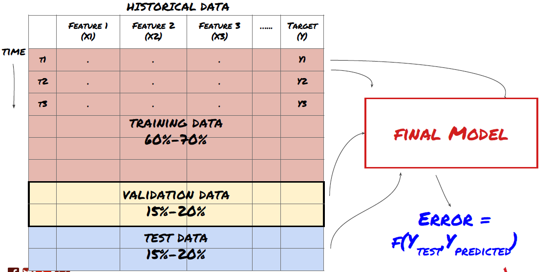
Step three: Split the data

• Create training sets from data, cross-validate and test these datasets

This is a very important step!Before we proceed, we should break the data into training datasets to train your model; test datasets to evaluate model performance. It is recommended to break the data into: 60-70% training sets and 30-40% test sets.

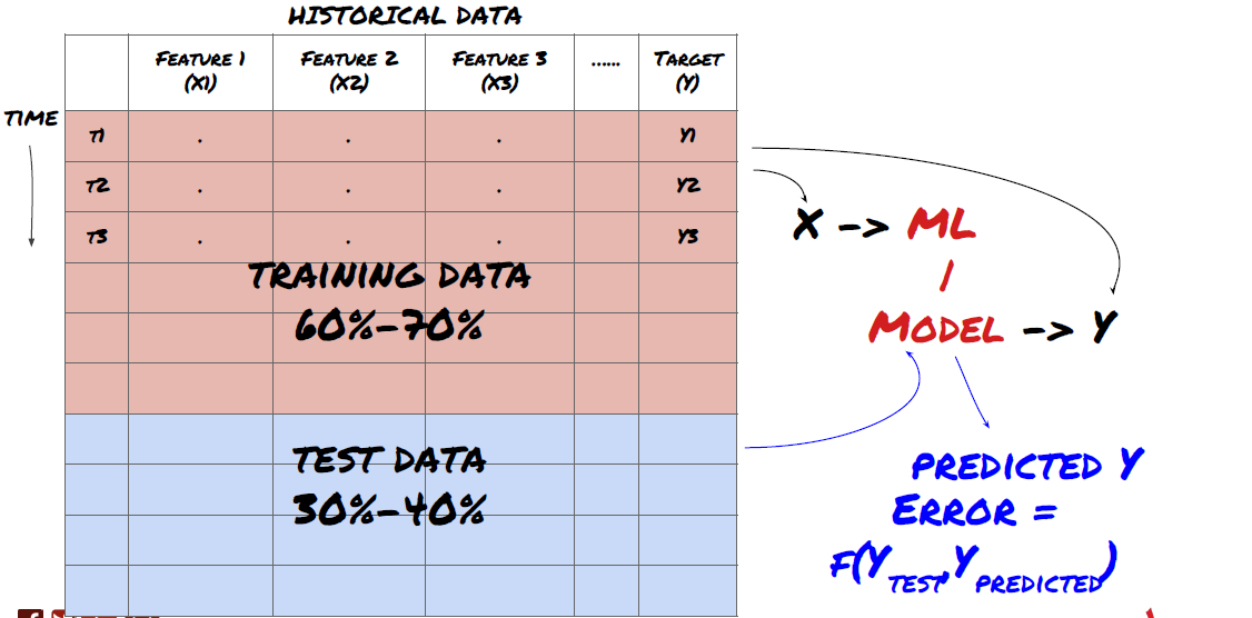
Split data into training sets and test sets

Since training data is used to evaluate model parameters, your model may over-fit these training data, and the training data may mislead model performance. If you don't keep any separate test data and use all of the data to train, you won't know how well or poorly your model performs on new unseen data. This is one of the main reasons why trained ML models fail with real-time data: people train all of the available data and get excited about the training data metrics, but the model can't make any meaningful predictions on untrained real-time data.

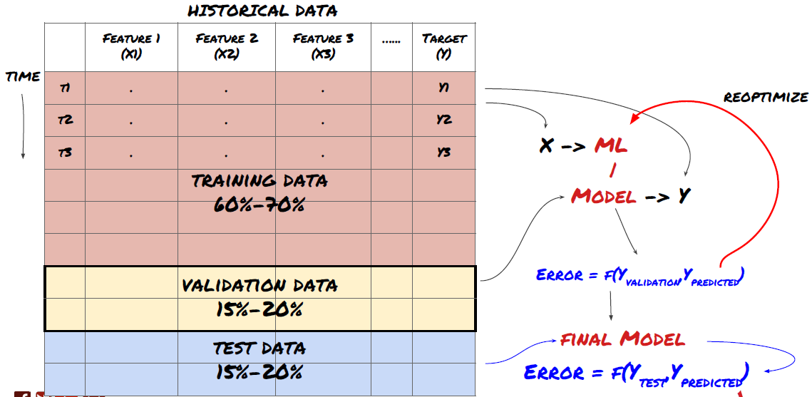
Break down data into training sets, validation sets, and test sets

There is a problem with this approach. If we repeatedly train training data, evaluate the performance of the test data, and optimize our model until we are satisfied with the performance, we implicitly include the test data as part of the training data. Ultimately, our model may perform well on this set of training and test data, but there is no guarantee that it will predict the new data well.

To solve this problem, we can create a separate verification dataset. Now, you can train the data, evaluate the performance of the verification data, optimize until you are satisfied with the performance, and finally test the test data. This way, the test data is not contaminated, and we do not use any information from the test data to improve our model.

Remember that once you have checked the performance of the test data, do not go back and try to optimize the model further. If you find that your model does not give good results, completely discard the model and start again. It is recommended to break it up into 60% training data, 20% validation data and 20% test data.

For our problem, we have three data sets available, and we will use one as our training set, the second as our verification set, and the third as our test set.

# Training Data
dataSetId =  'trainingData1'
ds_training = QuantQuestDataSource(cachedFolderName=cachedFolderName,
                                    dataSetId=dataSetId,
                                    instrumentIds=instrumentIds)
training_data = loadData(ds_training)
# Validation Data
dataSetId =  'trainingData2'
ds_validation = QuantQuestDataSource(cachedFolderName=cachedFolderName,
                                    dataSetId=dataSetId,
                                    instrumentIds=instrumentIds)
validation_data = loadData(ds_validation)
# Test Data
dataSetId =  'trainingData3'
ds_test = QuantQuestDataSource(cachedFolderName=cachedFolderName,
                                    dataSetId=dataSetId,
                                    instrumentIds=instrumentIds)
out_of_sample_test_data = loadData(ds_test)

For each of these, we add the target variable Y, defined as the average of the next five basis values.

def prepareData(data, period):
    data['Y(Target)'] = data['basis'].rolling(period).mean().shift(-period)
    if 'FairValue' in data.columns:
        del data['FairValue']
    data.dropna(inplace=True)
period = 5
prepareData(training_data, period)
prepareData(validation_data, period)
prepareData(out_of_sample_test_data, period)

Step four: Characterization

Analyze data behavior and create predictive features

Now the real engineering has begun. The golden rule of feature selection is that predictive power comes primarily from features, not from models. You will find that feature selection has a far greater impact on performance than model selection.

• Don't just pick a bunch of traits without exploring the relationship to the target variable.

• Very little or no relevance to the target variable may lead to overmatching

• The features you choose may be highly correlated with each other, in which case a smaller number of features can also explain the goal.

• I usually create some intuitive attributes to see how the target variables relate to these attributes and how they relate to each other to decide which ones to use.

• You can also try sorting candidate traits by maximum information coefficient (MIC), performing principal component analysis (PCA) and other methods.

This is the first time that the project has been implemented.

ML models tend to perform well when it comes to standardization. However, when dealing with time series data, standardization is tricky because the future range of data is unknown. Your data may go beyond the standardized range, leading to model errors.

• Scaling: characterized by standard deviation or four-digit range

• Residence: Subtract historical average from current value

• Unification: two regression periods of the above ((x - mean) /stdev)

• Conventional Unification: Standardize the data to a range of -1 to +1 and re-define the center in the regression period ((x-min) / ((max-min))

Note that because we use historical continuous averages, standard deviations, maximum values, or minimum values over the retrograde period, the standardized value of the attribute will represent different actual values at different times. For example, if the current value of the attribute is 5, the average of 30 consecutive cycles is 4.5, which will be converted to 0.5 after the interval; after that, if the mean of 30 consecutive cycles becomes 3, the value of 3.5 will become 0.5;; this may be the reason for model errors.

For the first iteration of our problem, we created a large number of features using the mixed parameters. Later we will try to see if we can reduce the number of features.

def difference(dataDf, period):
    return dataDf.sub(dataDf.shift(period), fill_value=0)
def ewm(dataDf, halflife):
    return dataDf.ewm(halflife=halflife, ignore_na=False,
                      min_periods=0, adjust=True).mean()
def rsi(data, period):
    data_upside = data.sub(data.shift(1), fill_value=0)
    data_downside = data_upside.copy()
    data_downside[data_upside > 0] = 0
    data_upside[data_upside < 0] = 0
    avg_upside = data_upside.rolling(period).mean()
    avg_downside = - data_downside.rolling(period).mean()
    rsi = 100 - (100 * avg_downside / (avg_downside + avg_upside))
    rsi[avg_downside == 0] = 100
    rsi[(avg_downside == 0) & (avg_upside == 0)] = 0
return rsi
def create_features(data):
    basis_X = pd.DataFrame(index = data.index, columns =  [])
    
    basis_X['mom3'] = difference(data['basis'],4)
    basis_X['mom5'] = difference(data['basis'],6)
    basis_X['mom10'] = difference(data['basis'],11)
    
    basis_X['rsi15'] = rsi(data['basis'],15)
    basis_X['rsi10'] = rsi(data['basis'],10)
    
    basis_X['emabasis3'] = ewm(data['basis'],3)
    basis_X['emabasis5'] = ewm(data['basis'],5)
    basis_X['emabasis7'] = ewm(data['basis'],7)
    basis_X['emabasis10'] = ewm(data['basis'],10)
    basis_X['basis'] = data['basis']
    basis_X['vwapbasis'] = data['stockVWAP']-data['futureVWAP']
    
    basis_X['swidth'] = data['stockTopAskPrice'] -
                        data['stockTopBidPrice']
    basis_X['fwidth'] = data['futureTopAskPrice'] -
                        data['futureTopBidPrice']
    
    basis_X['btopask'] = data['stockTopAskPrice'] -
                         data['futureTopAskPrice']
    basis_X['btopbid'] = data['stockTopBidPrice'] -
                         data['futureTopBidPrice']

    basis_X['totalaskvol'] = data['stockTotalAskVol'] -
                             data['futureTotalAskVol']
    basis_X['totalbidvol'] = data['stockTotalBidVol'] -
                             data['futureTotalBidVol']
    
    basis_X['emabasisdi7'] = basis_X['emabasis7'] -
                             basis_X['emabasis5'] + 
                             basis_X['emabasis3']
    
    basis_X = basis_X.fillna(0)
    
    basis_y = data['Y(Target)']
    basis_y.dropna(inplace=True)
    
    print("Any null data in y: %s, X: %s"
            %(basis_y.isnull().values.any(), 
             basis_X.isnull().values.any()))
    print("Length y: %s, X: %s"
            %(len(basis_y.index), len(basis_X.index)))
    
    return basis_X, basis_y
basis_X_train, basis_y_train = create_features(training_data)
basis_X_test, basis_y_test = create_features(validation_data)

Step five: Model selection

Select the appropriate statistical/ML model based on the question selected

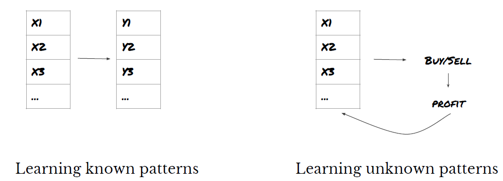
The choice of model depends on how the problem is constructed. Are you solving the supervised (each point X in the feature matrix is mapped to the target variable Y) or unsupervised learning problem (no mapping given, the model tries to learn the unknown pattern)? Are you solving the regression (actual price prediction at future time) or the classification problem (only price direction prediction at future time) (increase/decrease)).

Supervised or unsupervised learning

Regression or classification

Some common supervised learning algorithms can help you get started:

• Linear regression (parameter, regression) is the process of converting a linear regression into a linear regression.

• Logistic regression (parameters and classification)

• K-neighborhood (KNN) algorithm (example based, regression)

• SVM, SVR (parameters, classification and regression)

• The decision tree

• The Decision Forest

I suggest starting with a simple model, such as linear or logical regression, and building a more complex model from there as needed. I also suggest that you read the math behind the model rather than blindly using it as a black box.

Step 6: Training, verification and optimization (repeat steps 4-6)

Train and optimize your model using training and validation datasets

Now, you're ready to finally build the model. At this stage, you're really just iterating the model and model parameters. You train your model on the training data, measure its performance on the validation data, and then come back, optimize, retrain and evaluate.

Only when you have the model you like, then proceed to the next step.

For our presentation problem, let's start with a simple linear regression.

from sklearn import linear_model
from sklearn.metrics import mean_squared_error, r2_score
def linear_regression(basis_X_train, basis_y_train,
                      basis_X_test,basis_y_test):
    
    regr = linear_model.LinearRegression()
    # Train the model using the training sets
    regr.fit(basis_X_train, basis_y_train)
    # Make predictions using the testing set
    basis_y_pred = regr.predict(basis_X_test)
    # The coefficients
    print('Coefficients: \n', regr.coef_)
    
    # The mean squared error
    print("Mean squared error: %.2f"
          % mean_squared_error(basis_y_test, basis_y_pred))
    
    # Explained variance score: 1 is perfect prediction
    print('Variance score: %.2f' % r2_score(basis_y_test,
                                            basis_y_pred))
    # Plot outputs
    plt.scatter(basis_y_pred, basis_y_test,  color='black')
    plt.plot(basis_y_test, basis_y_test, color='blue', linewidth=3)
    plt.xlabel('Y(actual)')
    plt.ylabel('Y(Predicted)')
    plt.show()
    
    return regr, basis_y_pred
_, basis_y_pred = linear_regression(basis_X_train, basis_y_train, 
                                    basis_X_test,basis_y_test)

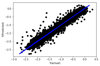
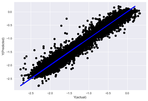
Linear regression without unification

('Coefficients: \n', array([ -1.0929e+08, 4.1621e+07, 1.4755e+07, 5.6988e+06, -5.656e+01, -6.18e-04, -8.2541e-05,4.3606e-02, -3.0647e-02, 1.8826e+07, 8.3561e-02, 3.723e-03, -6.2637e-03, 1.8826e+07, 1.8826e+07, 6.4277e-02, 5.7254e-02, 3.3435e-03, 1.6376e-02, -7.3588e-03, -8.1531e-04, -3.9095e-02, 3.1418e-02, 3.3321e-03, -1.3262e-06, -1.3433e+07, 3.5821e+07, 2.6764e+07, -8.0394e+06, -2.2388e+06, -1.7096e+07]))
Mean squared error: 0.02
Variance score: 0.96

Look at the model coefficients. We can't really compare them or say which ones are important because they all belong to different scales. Let's try to unify them so that they fit into the same proportions and also enforce some stability.

def normalize(basis_X, basis_y, period):
    basis_X_norm = (basis_X - basis_X.rolling(period).mean())/
                    basis_X.rolling(period).std()
    basis_X_norm.dropna(inplace=True)
    basis_y_norm = (basis_y - 
                    basis_X['basis'].rolling(period).mean())/
                    basis_X['basis'].rolling(period).std()
    basis_y_norm = basis_y_norm[basis_X_norm.index]
    
    return basis_X_norm, basis_y_norm
norm_period = 375
basis_X_norm_test, basis_y_norm_test = normalize(basis_X_test,basis_y_test, norm_period)
basis_X_norm_train, basis_y_norm_train = normalize(basis_X_train, basis_y_train, norm_period)
regr_norm, basis_y_pred = linear_regression(basis_X_norm_train, basis_y_norm_train, basis_X_norm_test, basis_y_norm_test)
basis_y_pred = basis_y_pred * basis_X_test['basis'].rolling(period).std()[basis_y_norm_test.index] + basis_X_test['basis'].rolling(period).mean()[basis_y_norm_test.index]

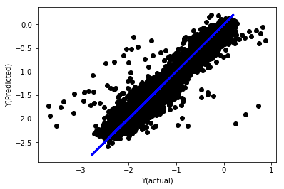
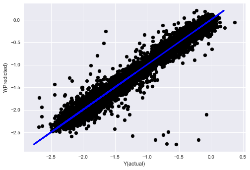
Linear regression of unification

Mean squared error: 0.05
Variance score: 0.90

The model does not improve on the previous model, but it is not worse. Now we can actually compare the coefficients and see which coefficients actually matter.

Let's look at the coefficients.

for i in range(len(basis_X_train.columns)):
    print('%.4f, %s'%(regr_norm.coef_[i], basis_X_train.columns[i]))

The results were:

19.8727, emabasis4
-9.2015, emabasis5
8.8981, emabasis7
-5.5692, emabasis10
-0.0036, rsi15
-0.0146, rsi10
0.0196, mom10
-0.0035, mom5
-7.9138, basis
0.0062, swidth
0.0117, fwidth
2.0883, btopask
2.0311, btopbid
0.0974, bavgask
0.0611, bavgbid
0.0007, topaskvolratio
0.0113, topbidvolratio
-0.0220, totalaskvolratio
0.0231, totalbidvolratio

We can clearly see that some traits have higher coefficients than others and may be more predictive.

Let's look at the correlation between the different traits.

import seaborn

c = basis_X_train.corr()
plt.figure(figsize=(10,10))
seaborn.heatmap(c, cmap='RdYlGn_r', mask = (np.abs(c) <= 0.8))
plt.show()

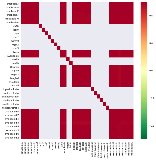
Correlation between features

The dark red area represents the highly relevant variable. Let's create/modify some features again and try to improve our model.

例如，我可以轻松地丢弃像emabasisdi7这样的特征，这些特征只是其他特征的线性组合.

def create_features_again(data):
    basis_X = pd.DataFrame(index = data.index, columns =  [])
    basis_X['mom10'] = difference(data['basis'],11)
    basis_X['emabasis2'] = ewm(data['basis'],2)
    basis_X['emabasis5'] = ewm(data['basis'],5)
    basis_X['emabasis10'] = ewm(data['basis'],10)
    basis_X['basis'] = data['basis']
    basis_X['totalaskvolratio'] = (data['stockTotalAskVol']
                                 - data['futureTotalAskVol'])/
                                   100000
    basis_X['totalbidvolratio'] = (data['stockTotalBidVol']
                                 - data['futureTotalBidVol'])/
                                   100000
    basis_X = basis_X.fillna(0)
    
    basis_y = data['Y(Target)']
    basis_y.dropna(inplace=True)
    return basis_X, basis_y
basis_X_test, basis_y_test = create_features_again(validation_data)
basis_X_train, basis_y_train = create_features_again(training_data)
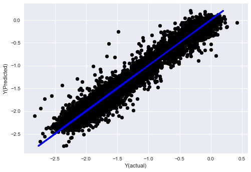
_, basis_y_pred = linear_regression(basis_X_train, basis_y_train, basis_X_test,basis_y_test)
basis_y_regr = basis_y_pred.copy()

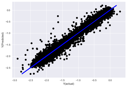
('Coefficients: ', array([ 0.03246139,
0.49780982, -0.22367172,  0.20275786,  0.50758852,
-0.21510795, 0.17153884]))
Mean squared error: 0.02
Variance score: 0.96

Look, our model performance hasn't changed, we just need some features to explain our target variable. I suggest you try more of the features above, try new combinations, etc., and see what can be improved on our model.

我们还可以尝试更复杂的模型，看看模型的变化是否可以提高性能.

• K-neighbor (KNN) algorithm

from sklearn import neighbors
n_neighbors = 5
model = neighbors.KNeighborsRegressor(n_neighbors, weights='distance')
model.fit(basis_X_train, basis_y_train)
basis_y_pred = model.predict(basis_X_test)
basis_y_knn = basis_y_pred.copy()

• SVR

from sklearn.svm import SVR
model = SVR(kernel='rbf', C=1e3, gamma=0.1)
model.fit(basis_X_train, basis_y_train)
basis_y_pred = model.predict(basis_X_test)
basis_y_svr = basis_y_pred.copy()

• The decision tree

model=ensemble.ExtraTreesRegressor()
model.fit(basis_X_train, basis_y_train)
basis_y_pred = model.predict(basis_X_test)
basis_y_trees = basis_y_pred.copy()

Step 7: Reassess the test data

Check the performance of actual sample data

Retest performance on the test dataset (not yet touched)

This is the critical moment. We start from the last step of the test data to run our final optimization model, we put it aside at the beginning, the data that has not been touched so far.

This gives you a realistic expectation of how your model will execute on new and unseen data when you start trading in real-time. It is therefore necessary to ensure that you have a clean dataset that is not used to train or validate the model.

If you don't like the results of the retest of the test data, please discard the model and start again. Never go back to re-optimizing your model, this will lead to over-fit! (It is also recommended to create a new test dataset, as this dataset has now been contaminated; we already know implicitly what the data set is about when we discard the model.)

So here we're going to use the Auquan's toolbox.

import backtester
from backtester.features.feature import Feature
from backtester.trading_system import TradingSystem
from backtester.sample_scripts.fair_value_params import FairValueTradingParams
class Problem1Solver():
def getTrainingDataSet(self):
        return "trainingData1"
def getSymbolsToTrade(self):
        return ['MQK']
def getCustomFeatures(self):
        return {'my_custom_feature': MyCustomFeature}
def getFeatureConfigDicts(self):
                            
        expma5dic = {'featureKey': 'emabasis5',
                 'featureId': 'exponential_moving_average',
                 'params': {'period': 5,
                              'featureName': 'basis'}}
        expma10dic = {'featureKey': 'emabasis10',
                 'featureId': 'exponential_moving_average',
                 'params': {'period': 10,
                              'featureName': 'basis'}}                     
        expma2dic = {'featureKey': 'emabasis3',
                 'featureId': 'exponential_moving_average',
                 'params': {'period': 3,
                              'featureName': 'basis'}}
        mom10dic = {'featureKey': 'mom10',
                 'featureId': 'difference',
                 'params': {'period': 11,
                              'featureName': 'basis'}}
        
        return [expma5dic,expma2dic,expma10dic,mom10dic]    
    
    def getFairValue(self, updateNum, time, instrumentManager):
        # holder for all the instrument features
        lbInstF = instrumentManager.getlookbackInstrumentFeatures()
        mom10 = lbInstF.getFeatureDf('mom10').iloc[-1]
        emabasis2 = lbInstF.getFeatureDf('emabasis2').iloc[-1]
        emabasis5 = lbInstF.getFeatureDf('emabasis5').iloc[-1]
        emabasis10 = lbInstF.getFeatureDf('emabasis10').iloc[-1] 
        basis = lbInstF.getFeatureDf('basis').iloc[-1]
        totalaskvol = lbInstF.getFeatureDf('stockTotalAskVol').iloc[-1] - lbInstF.getFeatureDf('futureTotalAskVol').iloc[-1]
        totalbidvol = lbInstF.getFeatureDf('stockTotalBidVol').iloc[-1] - lbInstF.getFeatureDf('futureTotalBidVol').iloc[-1]
        
        coeff = [ 0.03249183, 0.49675487, -0.22289464, 0.2025182, 0.5080227, -0.21557005, 0.17128488]
        newdf['MQK'] = coeff[0] * mom10['MQK'] + coeff[1] * emabasis2['MQK'] +\
                      coeff[2] * emabasis5['MQK'] + coeff[3] * emabasis10['MQK'] +\
                      coeff[4] * basis['MQK'] + coeff[5] * totalaskvol['MQK']+\
                      coeff[6] * totalbidvol['MQK']
                    
        newdf.fillna(emabasis5,inplace=True)
        return newdf
problem1Solver = Problem1Solver()
tsParams = FairValueTradingParams(problem1Solver)
tradingSystem = TradingSystem(tsParams)
tradingSystem.startTrading(onlyAnalyze=False, 
                           shouldPlot=True,
                           makeInstrumentCsvs=False)

Re-test results, Pnl calculated in USD (Pnl excludes transaction costs and other fees)

Step 8: Other ways to improve the model

Scroll verification, group learning, bagging and boosting

In addition to collecting more data, creating better features, or trying more models, there are a few things you can try to improve.

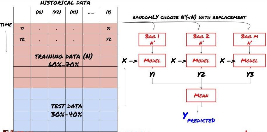
1. Scroll through verification

Scrolling through verification

Market conditions rarely stay the same. Assuming you have a year's worth of data and you train with data from January to August and use data from September to December to test your model, you may end up training against a very specific set of market conditions. Perhaps the first half of the year is free of market volatility, some extreme news causes the market to rise sharply in September, your model can't learn the pattern, and it will give you junk predictions.

It may be better to try forward rolling verification with January to February training, March verification, April to May retraining, June verification, etc.

2. Collective learning

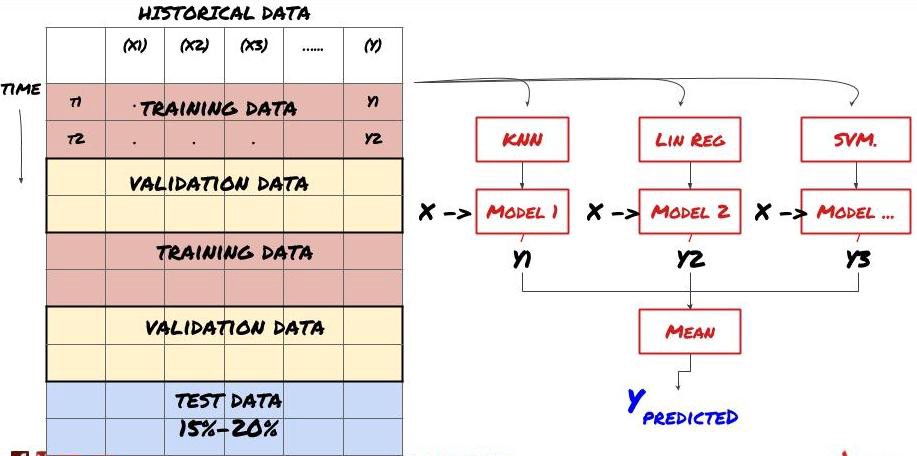
Collective learning

Some models may perform well in predicting certain scenarios, while others may be extremely overmatched or in some cases the model may be extremely overmatched. One way to reduce errors and overmatches is to use a set of different models. Your prediction will be the average of the predictions made by many models, and the errors of the different models may be offset or reduced.

Bagging

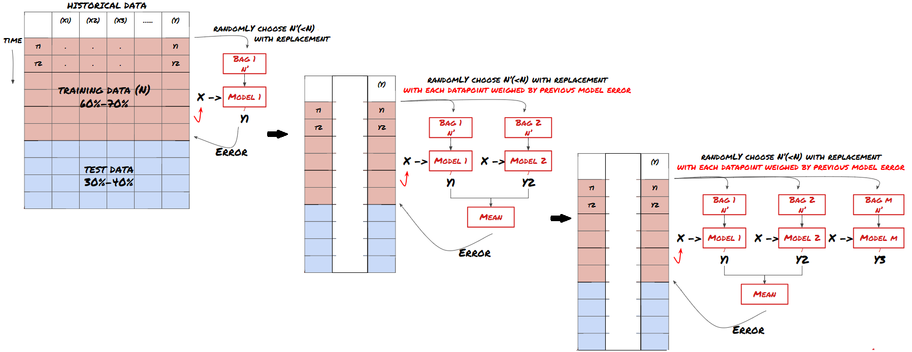
Boosting

For the sake of brevity, I'll skip these methods, but you can find more information online.

So let's try an aggregate approach to our problem.

basis_y_pred_ensemble = (basis_y_trees + basis_y_svr +
                         basis_y_knn + basis_y_regr)/4

Mean squared error: 0.02
Variance score: 0.95

So far, we have accumulated a lot of knowledge and information. Let's take a quick look back:

• Solving Your Problems

• Collect reliable data and clean up data

• Break down data into training, validation and test sets

• Creating traits and analyzing their behavior

• Choosing the right training model based on behavior

• Use training data to train your model and make predictions

• Check and re-optimize performance on the verification set

• Verify the final performance of the test set

But it's not over yet, you only have one reliable prediction model now. Remember what we really want in our strategy?

• Developing predictive model-based signals to identify trade direction

• Developing specific strategies to identify open positions

• Execution system to identify positions and prices

This is the inventor's quantification platform.FMZ.COMInventor's Quantify platform, there are many well-established alternative strategies, including the machine learning methodology in this article, that will make your specific strategy like a tiger wing. Strategy Square is located:https://www.fmz.com/square

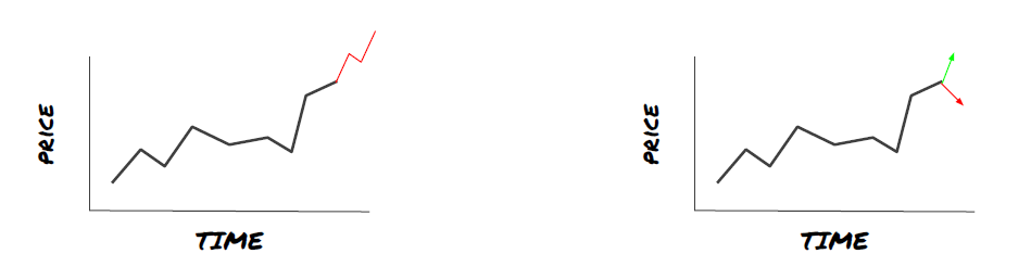
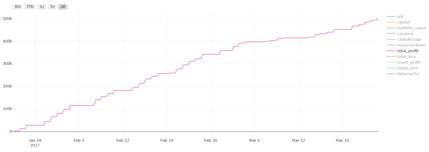
Important information about transaction costs：你的模型会告诉你所选资产何时是做多或做空。然而，它没有考虑费用/交易成本/可用交易量/止损等。交易成本通常会使有利可图的交易成为亏损。例如，预期价格上涨0.05美元的资产是买入，但如果你必须支付0.10美元进行此交易，你将最终获得净亏损$0.05。在你考虑经纪人佣金，交换费和点差后，我们上面看起来很棒的盈利图实际上是这样的：

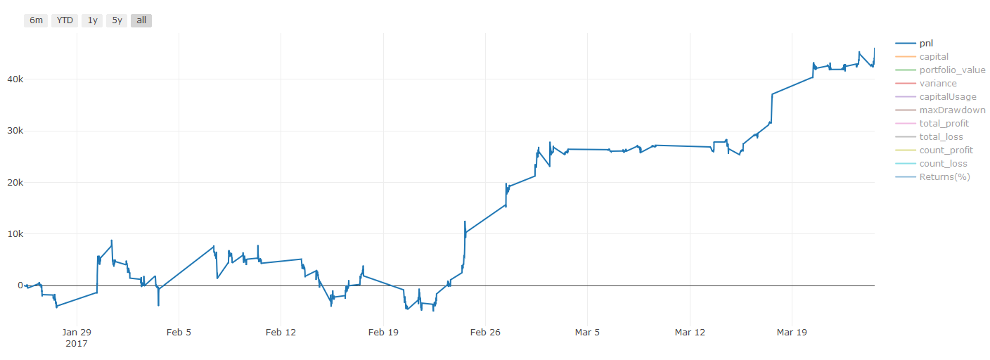
Pnl in US dollars after transaction fees and marginal returns

The transaction fees and spreads account for more than 90% of our PNL!

Finally, let's look at some common pitfalls.

What to do and what not to do

• Do your best to avoid over-fitting!

• Do not retrain after each data point: this is a common mistake people make in machine learning development. If your model needs to retrain after each data point, then it is probably not a very good model. That is, it needs to retrain regularly and only at a reasonable frequency (e.g. if you are doing a forecast during the day, retrain at the end of each week)

• Avoid biases, especially forward biases: This is another reason for the model not to work, make sure you don't use any future information. In most cases, this means not using the target variable Y as a feature in the model. You can use it during retrograde testing, but it won't be available when the model is actually running, which will render your model unusable.

• Beware of data mining biases: Since we are trying to model our data in a series of ways to determine its suitability, if there is no particular reason for this, make sure you run rigorous tests to separate the random pattern from the actual patterns that might occur. For example, linear regression explains well the uptrend pattern, which is only likely to be a small fraction of the larger random drift!

Avoid over-fitting

This is very important, and I feel it necessary to mention it again.

• Overfitting is the most dangerous trap in trading strategies

• A sophisticated algorithm may perform very well in retrospect, but it fails miserably in new, invisible data, which does not really reveal any trends in the data, nor does it have any real predictive power. It is well suited to the data it sees.

• Keep your system as simple as possible. If you find yourself needing a lot of complex functions to interpret data, you may be over-compliant.

• Break down your available data into training and test data, and always verify the performance of the actual sample data before using the model for real-time trading.

Related

More