ARMA-EGARCH 모델을 기반으로 비트코인 변동성의 모델링 및 분석

최근에, 나는 Bitcoin의 변동성에 대한 분석을 한 적이 있는데, 그것은 단어적이고 자발적입니다. 그래서 나는 단순히 내 이해와 코드를 다음과 같이 공유합니다. 내 능력은 제한되어 있으며 코드는 매우 완벽하지 않습니다. 어떤 오류가있는 경우, 그것을 지적하고 직접 수정하십시오.

1. 금융의 시간 계열에 대한 간략한 설명

금융의 시간 계열은 시간 차원에서 관찰되는 변수에 기반한 스토카스틱 프로세스 시리즈 모델의 집합이다. 변수는 일반적으로 자산의 수익률이다. 수익률은 투자 규모와 독립적이며 통계적 성격을 가지고 있기 때문에 기본 금융 자산의 투자 기회를 분석하는 것이 더 가치있다.

여기서는 비트코인의 수익률이 일반 금융 자산의 수익률 특성에 부합한다는 것을 대담하게 가정합니다. 즉, 그것은 몇 개의 샘플의 일관성 테스트를 통해 입증 할 수있는 약하게 부드러운 일련입니다.

1-1. 준비물, 수입 라이브러리, 캡슐화 기능

연구 환경의 구성이 완료되었습니다. 후속 계산에 필요한 라이브러리는 여기에 수입됩니다. 간헐적으로 작성되기 때문에 불필요한 것일 수 있습니다. 직접 청소하십시오.

[1]에서:

'''
start: 2020-02-01 00:00:00
end: 2020-03-01 00:00:00
period: 1h
exchanges: [{"eid":"Huobi","currency":"BTC_USDT","stocks":0}]
'''
from __future__ import absolute_import, division, print_function
from fmz import * # Import all FMZ functions
import pandas as pd
import numpy as np
import matplotlib.pyplot as plt
import matplotlib.lines as mlines
import seaborn as sns
import statsmodels.api as sm
import statsmodels.formula.api as smf
import statsmodels.tsa.api as smt
from statsmodels.graphics.api import qqplot
from statsmodels.stats.diagnostic import acorr_ljungbox as lb_test
from scipy import stats
from arch import arch_model
from datetime import timedelta
from itertools import product
from math import sqrt
from sklearn.metrics import r2_score, mean_absolute_error, mean_squared_error

task = VCtx(__doc__) # Initialization, verification of FMZ reading of historical data
print(exchange.GetAccount())

외출 [1]: {조금: 10000.0, 냉금: 0.0, 주식: 0.0, 냉금: 0.0}

    #### Encapsulate some of the functions, which will be used later. If there is a source, see the note

[17]에서:

# Plot functions
def tsplot(y, y_2, lags=None, title='', figsize=(18, 8)):  # source code: https://tomaugspurger.github.io/modern-7-timeseries.html
    fig = plt.figure(figsize=figsize)
    layout = (2, 2)
    ts_ax   = plt.subplot2grid(layout, (0, 0))
    ts2_ax = plt.subplot2grid(layout, (0, 1))
    acf_ax  = plt.subplot2grid(layout, (1, 0))
    pacf_ax = plt.subplot2grid(layout, (1, 1))
    y.plot(ax=ts_ax)
    ts_ax.set_title(title)
    y_2.plot(ax=ts2_ax)
    smt.graphics.plot_acf(y, lags=lags, ax=acf_ax)
    smt.graphics.plot_pacf(y, lags=lags, ax=pacf_ax)
    [ax.set_xlim(0) for ax in [acf_ax, pacf_ax]]
    sns.despine()
    plt.tight_layout()
    return ts_ax, ts2_ax, acf_ax, pacf_ax

# Performance evaluation
def get_rmse(y, y_hat):
    mse = np.mean((y - y_hat)**2)
    return np.sqrt(mse)

def get_mape(y, y_hat):
    perc_err = (100*(y - y_hat))/y
    return np.mean(abs(perc_err))

def get_mase(y, y_hat):
    abs_err = abs(y - y_hat)
    dsum=sum(abs(y[1:] - y_hat[1:]))
    t = len(y)
    denom = (1/(t - 1))* dsum
    return np.mean(abs_err/denom)

def mae(observation, forecast):    
    error = mean_absolute_error(observation, forecast)
    print('Mean Absolute Error (MAE): {:.3g}'.format(error))
    return error

def mape(observation, forecast): 
    observation, forecast = np.array(observation), np.array(forecast)
    # Might encounter division by zero error when observation is zero
    error = np.mean(np.abs((observation - forecast) / observation)) * 100
    print('Mean Absolute Percentage Error (MAPE): {:.3g}'.format(error))
    return error

def rmse(observation, forecast):
    error = sqrt(mean_squared_error(observation, forecast))
    print('Root Mean Square Error (RMSE): {:.3g}'.format(error))
    return error

def evaluate(pd_dataframe, observation, forecast):
    first_valid_date = pd_dataframe[forecast].first_valid_index()
    mae_error = mae(pd_dataframe[observation].loc[first_valid_date:, ], pd_dataframe[forecast].loc[first_valid_date:, ])
    mape_error = mape(pd_dataframe[observation].loc[first_valid_date:, ], pd_dataframe[forecast].loc[first_valid_date:, ])
    rmse_error = rmse(pd_dataframe[observation].loc[first_valid_date:, ], pd_dataframe[forecast].loc[first_valid_date:, ]) 

    ax = pd_dataframe.loc[:, [observation, forecast]].plot(figsize=(18,5))
    ax.xaxis.label.set_visible(False)
    return

1-2. 비트코인의 역사적인 데이터에 대한 간략한 이해로 시작합시다.

통계적 관점에서, 우리는 비트코인의 몇 가지 데이터 특성을 살펴볼 수 있다. 예를 들어 지난 해의 데이터 설명을 들자면, 수익률은 간단한 방법으로 계산된다. 즉, 폐쇄 가격은 로그아리듬적으로 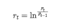니다. 공식은 다음과 같다:

[3]에서:

df = get_bars('huobi.btc_usdt', '1d', count=10000, start='2019-01-01')
btc_year = pd.DataFrame(df['close'],dtype=np.float)
btc_year.index.name = 'date'
btc_year.index = pd.to_datetime(btc_year.index)
btc_year['log_price'] = np.log(btc_year['close'])
btc_year['log_return'] = btc_year['log_price'] - btc_year['log_price'].shift(1)
btc_year['log_return_100x'] = np.multiply(btc_year['log_return'], 100)

btc_year_test = pd.DataFrame(btc_year['log_return'].dropna(), dtype=np.float)
btc_year_test.index.name = 'date'
mean = btc_year_test.mean()
std = btc_year_test.std()
normal_result = pd.DataFrame(index=['Mean Value', 'Std Value', 'Skewness Value','Kurtosis Value'], columns=['model value'])
normal_result['model value']['Mean Value'] = ('%.4f'% mean[0])
normal_result['model value']['Std Value'] = ('%.4f'% std[0])
normal_result['model value']['Skewness Value'] = ('%.4f'% btc_year_test.skew())
normal_result['model value']['Kurtosis Value'] = ('%.4f'% btc_year_test.kurt())
normal_result

아웃[3]: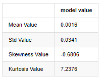

두꺼운 지방 꼬리의 특징은 시간 스케일이 짧을수록 특징이 더 중요합니다. 커토스는 데이터 주파수의 증가에 따라 증가 할 것이며, 특징은 고주파 데이터에서 매우 분명합니다.

2019년 1월 1일부터 현재까지의 일일 폐쇄 가격 데이터를 예로 들면, 우리는 그것의 로그아리듬적 수익률에 대한 서술적 분석을 하고, 비트코인의 단순한 수익률 시리즈가 정상적인 분포와 일치하지 않으며, 두꺼운 지방 꼬리의 명백한 특징을 가지고 있음을 볼 수 있습니다.

시퀀스의 평균 값은 0.0016, 표준편차는 0.0341, 편향은 -0.6819, 커토시스는 7.2243이며, 이는 정상적인 분포보다 훨씬 높으며 두꺼운 지방 꼬리의 특징을 가지고 있습니다. Bitcoin의 단순한 수익률의 정상성은 QQ 차트로 측정 및 테스트됩니다.

[4]:

fig = plt.figure(figsize=(4,4))
ax = fig.add_subplot(111)
fig = qqplot(btc_year_test['log_return'], line='q', ax=ax, fit=True)

아웃[4]:

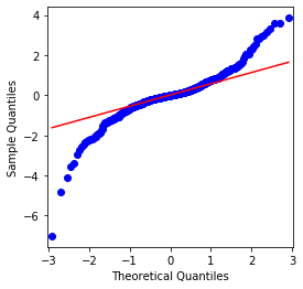
QQ 차트는 완벽하고 비트코인의 로그리듬적 환산 순서는 결과의 정상적인 분포에 맞지 않으며 두꺼운 뚱뚱한 꼬리라는 명백한 특징을 가지고 있습니다.

다음으로, 변동성 집계 효과를 살펴보자. 즉, 금융 시간 계열은 종종 더 큰 변동성 이후에 더 큰 변동성이 동반되며, 더 작은 변동성은 일반적으로 더 작은 변동성이 따라옵니다.

변동성 클러스터링은 변동성의 긍정적 및 부정적인 피드백 효과를 반영하며 지방 꼬리 특성과 밀접한 상관관계를 가지고 있습니다. 경제학적으로 이것은 변동성의 시간 계열이 자동 상관관계를 가질 수 있음을 암시합니다. 즉, 현재 기간의 변동성은 이전 기간, 두 번째 이전 기간 또는 심지어 세 번째 이전 기간과 어떤 관계가있을 수 있습니다.

[5]에서:

df = get_bars('huobi.btc_usdt', '1d', count=50000, start='2006-01-01')
btc_year = pd.DataFrame(df['close'],dtype=np.float)
btc_year.index.name = 'date'
btc_year.index = pd.to_datetime(btc_year.index)
btc_year['log_price'] = np.log(btc_year['close'])
btc_year['log_return'] = btc_year['log_price'] - btc_year['log_price'].shift(1)
btc_year['log_return_100x'] = np.multiply(btc_year['log_return'], 100)

btc_year_test = pd.DataFrame(btc_year['log_return'].dropna(), dtype=np.float)
btc_year_test.index.name = 'date'
sns.mpl.rcParams['figure.figsize'] = (18, 4)  # Volatility
ax1 = btc_year_test['log_return'].plot()
ax1.xaxis.label.set_visible(False)

외출[5]:

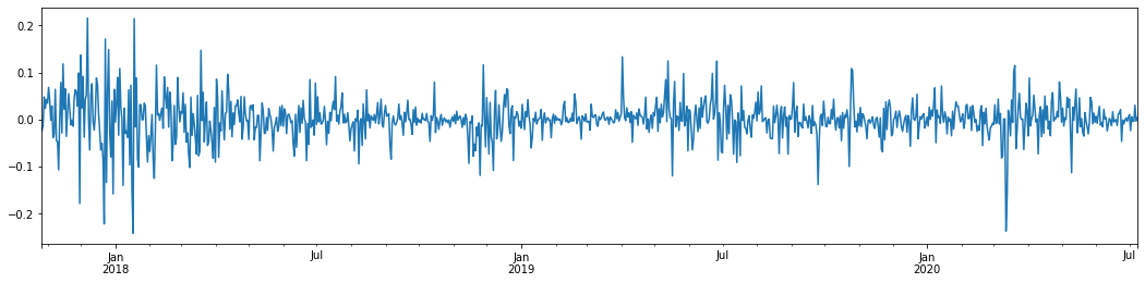
지난 3년 동안 비트코인의 일일 로그아리듬률 수익률을 추론해 보면 변동성 집합화 현상이 분명하게 나타난다. 2018년 비트코인의 황금시장 이후, 대부분의 기간 동안 안정적인 지위에 있었다. 극우에서 볼 수 있듯이, 2020년 3월, 글로벌 금융시장이 무너지면서 비트코인 유동성에도 러닝이 있었고, 수익률은 하루 동안 40% 가까이 급격히 떨어졌고, 급격한 부정적인 변동이 있었다.

한마디로, 직관적인 관찰에서, 우리는 큰 변동이 큰 확률로 밀도가 높은 변동에 의해 이어질 것을 볼 수 있습니다. 이는 또한 변동성의 집계 효과입니다. 이 변동성 범위가 예측 가능하다면 BTC의 단기 거래에 유용합니다. 이는 변동성을 논의하는 목적이기도 합니다.

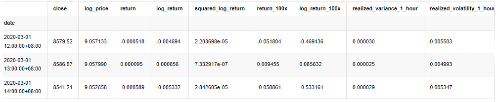
1-3. 데이터 준비

훈련 샘플 세트를 준비하기 위해 먼저, 우리는 리그리듬 수익률이 관찰된 변동성에 해당하는 벤치마크 샘플을 설정합니다. 하루의 변동성을 직접 관찰 할 수 없기 때문에 시간 데이터를 재 샘플링에 사용하여 하루의 실현 변동성을 추론하고 변동성의 의존 변수로 사용합니다.

재 샘플링 방법은 시간 데이터에 기초합니다. 공식은 다음과 같습니다.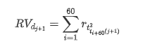

[4]:

count_num = 100000
start_date = '2020-03-01'

df = get_bars('huobi.btc_usdt', '1m', count=50000, start='2020-02-13')  # Take the minute data
kline_1m = pd.DataFrame(df['close'], dtype=np.float)
kline_1m.index.name = 'date'
kline_1m['log_price'] = np.log(kline_1m['close'])
kline_1m['return'] = kline_1m['close'].pct_change().dropna()
kline_1m['log_return'] = kline_1m['log_price'] - kline_1m['log_price'].shift(1)

kline_1m['squared_log_return'] = np.power(kline_1m['log_return'], 2)

kline_1m['return_100x'] = np.multiply(kline_1m['return'], 100)
kline_1m['log_return_100x'] = np.multiply(kline_1m['log_return'], 100)  # Enlarge 100 times

df = get_bars('huobi.btc_usdt', '1h', count=860, start='2020-02-13')  # Take the hour data
kline_all = pd.DataFrame(df['close'], dtype=np.float)
kline_all.index.name = 'date'
kline_all['log_price'] = np.log(kline_all['close'])  # Calculate daily logarithmic rate of return
kline_all['return'] = kline_all['log_price'].pct_change().dropna()
kline_all['log_return'] = kline_all['log_price'] - kline_all['log_price'].shift(1)  # Calculate logarithmic rate of return
kline_all['squared_log_return'] = np.power(kline_all['log_return'], 2)  # The exponential square of logarithmic daily rate of return

kline_all['return_100x'] = np.multiply(kline_all['return'], 100)
kline_all['log_return_100x'] = np.multiply(kline_all['log_return'], 100)  # Enlarge 100 times

kline_all['realized_variance_1_hour'] = kline_1m.loc[:, 'squared_log_return'].resample('h', closed='left', label='left').sum().copy()  # Resampling to days
kline_all['realized_volatility_1_hour'] = np.sqrt(kline_all['realized_variance_1_hour'])  # Volatility of variance derivation

kline_all = kline_all[4:-29] # Remove the last line because it is missing
kline_all.head(3)

아웃[4]: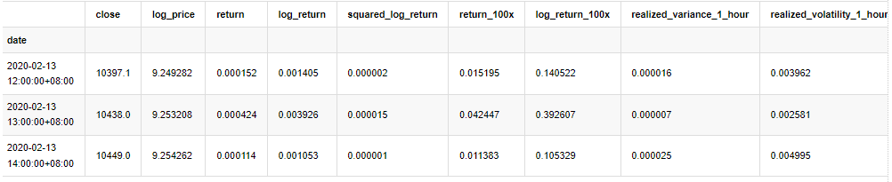

표본 밖의 데이터를 같은 방법으로 준비합니다.

[5]에서:

# Prepare the data outside the sample with realized daily volatility
df = get_bars('huobi.btc_usdt', '1m', count=50000, start='2020-02-13')  # Take the minute data
kline_1m = pd.DataFrame(df['close'], dtype=np.float)
kline_1m.index.name = 'date'
kline_1m['log_price'] = np.log(kline_1m['close'])
kline_1m['log_return'] = kline_1m['log_price'] - kline_1m['log_price'].shift(1)
kline_1m['log_return_100x'] = np.multiply(kline_1m['log_return'], 100)  # Enlarge 100 times
kline_1m['squared_log_return'] = np.power(kline_1m['log_return_100x'], 2)
kline_1m#.tail()
df = get_bars('huobi.btc_usdt', '1h', count=860, start='2020-02-13')  # Take the hour data
kline_test = pd.DataFrame(df['close'], dtype=np.float)
kline_test.index.name = 'date'
kline_test['log_price'] = np.log(kline_test['close'])  # Calculate daily logarithmic rate of return
kline_test['log_return'] = kline_test['log_price'] - kline_test['log_price'].shift(1)  # Calculate logarithmic rate of return
kline_test['log_return_100x'] = np.multiply(kline_test['log_return'], 100)  # Enlarge 100 times
kline_test['squared_log_return'] = np.power(kline_test['log_return_100x'], 2)  # The exponential square of logarithmic daily rate of return
kline_test['realized_variance_1_hour'] = kline_1m.loc[:, 'squared_log_return'].resample('h', closed='left', label='left').sum()  # Resampling to days
kline_test['realized_volatility_1_hour'] = np.sqrt(kline_test['realized_variance_1_hour'])  # Volatility of variance derivation
kline_test = kline_test[4:-2]

표본의 기본 데이터를 이해하려면 다음과 같이 간단한 설명적 분석을 수행합니다.

[9]에서:

line_test = pd.DataFrame(kline_train['log_return'].dropna(), dtype=np.float)
line_test.index.name = 'date'

mean = line_test.mean()  # Calculate mean value and standard deviation
std = line_test.std()

line_test.sort_values(by = 'log_return', inplace = True)  # Resort
s_r = line_test.reset_index(drop = False)  # After resorting, update index
s_r['p'] = (s_r.index - 0.5) / len(s_r)  # Calculate the percentile p(i)
s_r['q'] = (s_r['log_return'] - mean) / std  # Calculate the value of q

st = line_test.describe()
x1 ,y1 = 0.25, st['log_return']['25%']
x2 ,y2 = 0.75, st['log_return']['75%']

fig = plt.figure(figsize = (18,8))
layout = (2, 2)
ax1 = plt.subplot2grid(layout, (0, 0), colspan=2)# Plot the data distribution
ax2 = plt.subplot2grid(layout, (1, 0))# Plot histogram
ax3 = plt.subplot2grid(layout, (1, 1))# Draw the QQ chart, the straight line is the connection of the quarter digit, three-quarters digit, which is basically conforms to the normal distribution

ax1.scatter(line_test.index, line_test.values)
line_test.hist(bins=30,alpha = 0.5,ax = ax2)
line_test.plot(kind = 'kde', secondary_y=True,ax = ax2)
ax3.plot(s_r['p'],s_r['log_return'],'k.',alpha = 0.1)
ax3.plot([x1,x2],[y1,y2],'-r')
sns.despine()
plt.tight_layout()

아웃[9]:

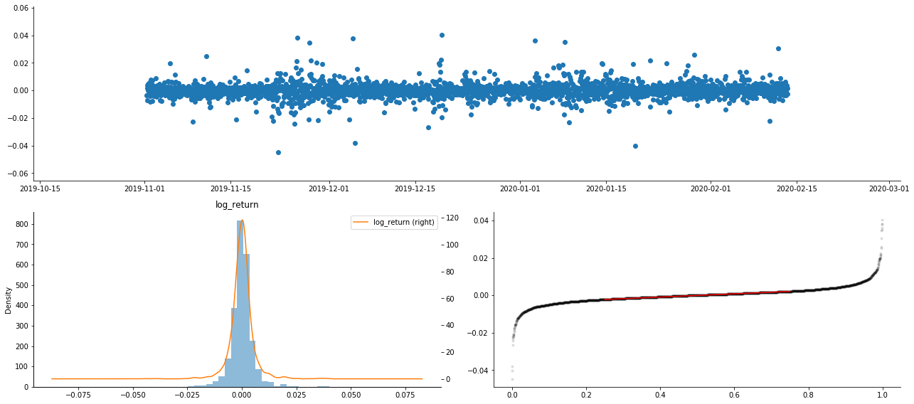
결과적으로, 로그아리듬 수익의 시간 계열 차트에는 명백한 변동성 집계와 레버리지 효과가 있습니다.

로그리즘 반환의 분포 차트의 편향은 0보다 작으며, 샘플의 반환이 약간 부정적이고 오른쪽으로 편향되어 있음을 나타냅니다. 로그리즘 반환의 QQ 차트에서 로그리즘 반환의 분포가 정상적이지 않다는 것을 볼 수 있습니다.

데이터 분포의 편향성은 1보다 작으며 표본 내의 반환이 약간 긍정적이고 약간 오른쪽으로 편향되어 있음을 나타냅니다. 커토시스 값은 3보다 크며 수익이 두꺼운 지방 꼬리 분포를 나타냅니다.

이제 우리가 이 지점에 도달했을 때, 또 다른 통계적 테스트를 해 봅시다. [7]에서:

line_test = pd.DataFrame(kline_all['log_return'].dropna(), dtype=np.float)
line_test.index.name = 'date'
mean = line_test.mean()
std = line_test.std()
normal_result = pd.DataFrame(index=['Mean Value', 'Std Value', 'Skewness Value','Kurtosis Value',
                                    'Ks Test Value','Ks Test P-value',
                                    'Jarque Bera Test','Jarque Bera Test P-value'],
                    columns=['model value'])
normal_result['model value']['Mean Value'] = ('%.4f'% mean[0])
normal_result['model value']['Std Value'] = ('%.4f'% std[0])
normal_result['model value']['Skewness Value'] = ('%.4f'% line_test.skew())
normal_result['model value']['Kurtosis Value'] = ('%.4f'% line_test.kurt())
normal_result['model value']['Ks Test Value'] = stats.kstest(line_test, 'norm', (mean, std))[0]
normal_result['model value']['Ks Test P-value'] = stats.kstest(line_test, 'norm', (mean, std))[1]
normal_result['model value']['Jarque Bera Test'] = stats.jarque_bera(line_test)[0]
normal_result['model value']['Jarque Bera Test P-value'] = stats.jarque_bera(line_test)[1]
normal_result

아웃[7]:

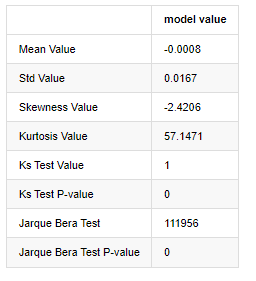
콜모고로프 - 스미르노프 및 자르크 - 베라 테스트 통계는 각각 사용됩니다. 원래 가설은 상당한 차이와 정상적인 분포로 특징입니다. P 값이 0.05% 신뢰 수준의 중요한 값보다 작으면 원래 가설은 거부됩니다.

커토시스 값이 3보다 크다는 것을 볼 수 있으며, 두꺼운 지방 꼬리의 특성을 나타냅니다. KS와 JB의 P 값은 신뢰도 간격보다 작습니다. 정상적인 분포의 가정이 거부되며 BTC의 수익률이 정상적인 분포의 특성을 가지고 있지 않으며 경험적 연구는 두꺼운 지방 꼬리의 특성을 가지고 있음을 증명합니다.

1-4. 실제 변동성과 관찰된 변동성의 비교

우리는 관측을 위해 squared_log_return (logarithmic yield squared) 와 realized_variance (realized variance) 를 결합합니다.

[11]에서:

fig, ax = plt.subplots(figsize=(18, 6))
start = '2020-03-08 00:00:00+08:00'
end = '2020-03-20 00:00:00+08:00'

np.abs(kline_all['squared_log_return']).loc[start:end].plot(ax=ax,label='squared log return')
kline_all['realized_variance_1_hour'].loc[start:end].plot(ax=ax,label='realized variance')
plt.legend(loc='best')

아웃[11]:

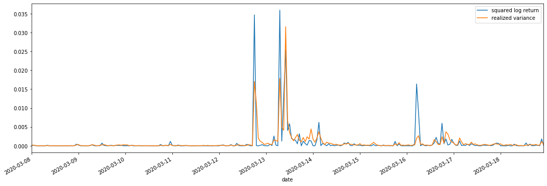
실현된 변동 범위가 커지면 수익률 범위의 변동성도 커지고 실현된 수익률이 부드럽다는 것을 알 수 있습니다. 둘 다 명백한 집계 효과를 관찰하기가 쉽습니다.

순수 이론적 관점에서, RV는 실제 변동성에 가깝고, 단기 변동성은 하루 내 변동성이 하루 하루 데이터에 속하기 때문에 평탄화됩니다. 따라서 관찰적 관점에서, 하루 내 변동성은 낮은 변동성 주식 시장 빈도에 더 적합합니다. 높은 빈도 거래 및 BTC의 7 * 24 시간 시장 특성은 RV를 벤치마크 변동성을 결정하는 데 더 적합하게 만듭니다.

2. 시간 계열 의 부드러움

만약 그것이 비정형 시리즈라면, 그것은 대략적으로 정형 시리즈로 조정되어야 한다. 일반적인 방법은 차이 처리를 하는 것이다. 이론적으로, 많은 차이의 후에, 비정형 시리즈는 정형 시리즈로 근사할 수 있다. 만약 표본 시리즈의 동변성이 안정적이라면, 그 관측의 기대, 동변성 및 동변성은 시간에 따라 변하지 않을 것이며, 표본 시리즈가 통계 분석에서 추론을 하기 위해 더 편리하다는 것을 나타낸다.

여기서 단위 뿌리 테스트, 즉 ADF 테스트가 사용된다. ADF 테스트는 중요성을 관찰하기 위해 t 테스트를 사용합니다. 원칙적으로, 시리즈가 명백한 추세를 보여주지 않으면 일정한 항목만 유지됩니다. 시리즈가 추세를 가지고 있다면 회귀 방정식은 일정한 항목과 시간 추세 항목을 모두 포함해야합니다. 또한 정보 기준에 기반한 평가에 AIC 및 BIC 기준을 사용할 수 있습니다. 공식이 필요한 경우 다음과 같습니다.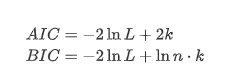

[8]에서:

stable_test = kline_all['log_return']
adftest = sm.tsa.stattools.adfuller(np.array(stable_test), autolag='AIC')
adftest2 = sm.tsa.stattools.adfuller(np.array(stable_test), autolag='BIC')
output=pd.DataFrame(index=['ADF Statistic Test Value', "ADF P-value", "Lags", "Number of Observations",
                           "Critical Value(1%)","Critical Value(5%)","Critical Value(10%)"],
                    columns=['AIC','BIC'])
output['AIC']['ADF Statistic Test Value'] = adftest[0]
output['AIC']['ADF P-value'] = adftest[1]
output['AIC']['Lags'] = adftest[2]
output['AIC']['Number of Observations'] = adftest[3]
output['AIC']['Critical Value(1%)'] = adftest[4]['1%']
output['AIC']['Critical Value(5%)'] = adftest[4]['5%']
output['AIC']['Critical Value(10%)'] = adftest[4]['10%']
output['BIC']['ADF Statistic Test Value'] = adftest2[0]
output['BIC']['ADF P-value'] = adftest2[1]
output['BIC']['Lags'] = adftest2[2]
output['BIC']['Number of Observations'] = adftest2[3]
output['BIC']['Critical Value(1%)'] = adftest2[4]['1%']
output['BIC']['Critical Value(5%)'] = adftest2[4]['5%']
output['BIC']['Critical Value(10%)'] = adftest2[4]['10%']
output

아웃[8]: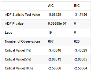

원래 가정은 일련에 단위 뿌리가 없다는 것입니다. 즉, 다른 가정은 일련이 정지 상태라는 것입니다. 테스트 P 값은 0.05% 신뢰 수준 절단 값보다 훨씬 적습니다. 원래 가정은 거부합니다. 따라서 로그 리턴 비율은 정지 일련이며 통계 시간 시리즈 모델을 사용하여 모델링 할 수 있습니다.

3. 모델 식별 및 주문 결정

평균값 방정식을 설정하기 위해서는 오류 단어가 자동 상관관계를 가지고 있지 않은지 확인하기 위해 순서에 대한 자동 상관관계 테스트를 수행해야합니다. 먼저 자동 상관관계 ACF와 부분 상관관계 PACF를 다음과 같이 그래프화하십시오.

[19]에서:

tsplot(kline_all['log_return'], kline_all['log_return'], title='Log Return', lags=100)

아웃[19]:

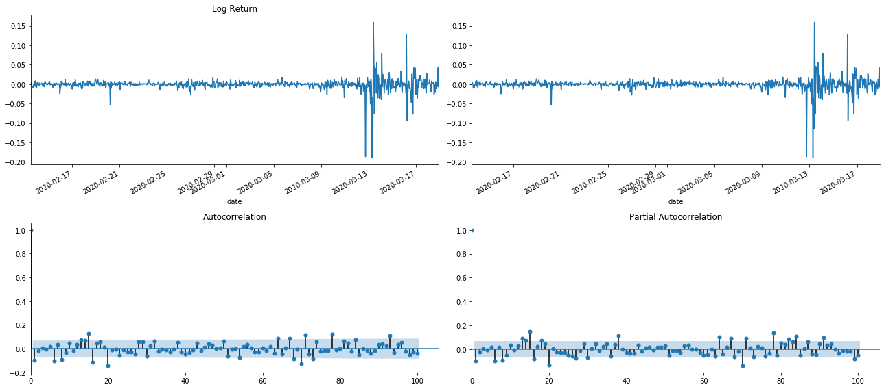
단축의 효과는 완벽하다는 것을 볼 수 있습니다. 그 순간에,이 그림은 저에게 영감을 주었습니다. 시장이 정말로 유효하지 않습니까? 확인하기 위해, 우리는 반환 시리즈에 대한 자동 상관 분석을 수행하고 모델의 지연 순서를 결정합니다.

일반적으로 사용되는 상관 계수는 자신과 그 사이의 상관 관계를 측정하는 것입니다. 즉 과거 특정 시간에 r (t) 와 r (t-l) 사이의 상관 관계를 측정합니다.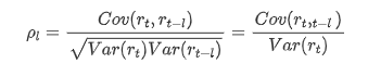

다음으로 양적 테스트를 해 봅시다. 원래 가정은 모든 자가 상관 계수가 0이라는 것입니다. 즉, 일련에 자가 상관 관계가 없습니다. 테스트 통계 공식은 다음과 같이 작성됩니다.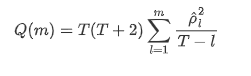

분석을 위해 다음과 같이 10 개의 자가 상관률을 취했습니다.

[9]에서:

acf,q,p = sm.tsa.acf(kline_all['log_return'], nlags=15,unbiased=True,qstat = True, fft=False)  # Test 10 autocorrelation coefficients
output = pd.DataFrame(np.c_[range(1,16), acf[1:], q, p], columns=['lag', 'ACF', 'Q', 'P-value'])
output = output.set_index('lag')
output

아웃[9]: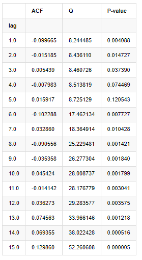

테스트 통계자료 Q와 P값에 따르면, 자동관계 함수 ACF가 순서 0 이후 점차 0이 되는 것을 볼 수 있다. Q 테스트 통계자료의 P값은 원래 가정을 거부할 만큼 작아서 일련에 자동관계가 있다.

4. ARMA 모델링

AR 및 MA 모델은 매우 간단합니다. 간단히 말해서, 마크다운은 공식을 작성하기에 너무 피곤합니다. 관심이 있다면 직접 확인하십시오. AR (자율 회귀) 모델은 주로 시간 계열을 모델링하는 데 사용됩니다. 계열이 ACF 테스트를 통과 한 경우, 즉 1의 간격으로 자동 상관 계수가 중요합니다. 즉, 시간에 대한 데이터는 시간 t를 예측하는 데 유용 할 수 있습니다.

MA (Moving Average) 모델은 현재 예측 값을 선형적으로 표현하기 위해 지난 q 기간의 무작위 간섭 또는 오류 예측을 사용합니다.

데이터의 동적 구조를 완전히 설명하기 위해서는 AR 또는 MA 모델의 순서를 높이는 것이 필요하지만 그러한 매개 변수는 계산을 더 복잡하게 만들 것입니다. 따라서이 프로세스를 단순화하기 위해 자가 회귀 이동 평균 (ARMA) 모델을 제안합니다.

가격 시간 계열은 일반적으로 정지적이지 않으며, 정지성에 대한 차이 방법의 최적화 효과는 이전에 논의되었기 때문에 ARIMA (p, d, q) (총량 자기 회전 이동 평균) 모델은 기존 모델의 일련의 적용을 기반으로 d 순위 차이 처리를 추가합니다. 그러나 로그리듬을 사용했기 때문에 ARMA (p, q) 를 직접 사용할 수 있습니다.

한마디로, ARIMA 모델과 ARMA 모델 구축 과정의 유일한 차이점은 정지성을 분석한 후 불안정한 결과를 얻으면 모델이 직접 시리즈에 제곱차 차이를 만들어 정지성 테스트를 수행하고 시리즈가 안정화 될 때까지 p와 q 순서를 결정한다는 것입니다. 모델을 구축하고 평가한 후, 그 다음 예측이 이루어지며, 차이를 다시 수행하는 단계를 제거합니다. 그러나 가격의 2 차 차 차 차이는 의미가 없기 때문에 ARMA는 최고의 선택입니다.

4-1 순서 선택

다음으로, 우리는 정보 기준에 의해 순서를 직접 선택할 수 있습니다. 여기 우리는 AIC와 BIC의 열역학 다이어그램으로 시도합니다.

[10]에서:

def select_best_params():
    ps = range(0, 4)
    ds= range(1, 2)
    qs = range(0, 4)
    parameters = product(ps, ds, qs)
    parameters_list = list(parameters)

    p_min = 0
    d_min = 0
    q_min = 0
    p_max = 3
    d_max = 3
    q_max = 3

    results_aic = pd.DataFrame(index=['AR{}'.format(i) for i in range(p_min,p_max+1)],
                               columns=['MA{}'.format(i) for i in range(q_min,q_max+1)])
    results_bic = pd.DataFrame(index=['AR{}'.format(i) for i in range(p_min,p_max+1)],
                               columns=['MA{}'.format(i) for i in range(q_min,q_max+1)])
    
    best_params = []
    aic_results = []
    bic_results = []
    hqic_results = []
    best_aic = float("inf")
    best_bic = float("inf")
    best_hqic = float("inf")
    warnings.filterwarnings('ignore')
    for param in parameters_list:
        try:
            model = sm.tsa.SARIMAX(kline_all['log_price'], order=(param[0], param[1], param[2])).fit(disp=-1)
            results_aic.loc['AR{}'.format(param[0]), 'MA{}'.format(param[2])] = model.aic
            results_bic.loc['AR{}'.format(param[0]), 'MA{}'.format(param[2])] = model.bic
        except ValueError:
            continue    
           
        aic_results.append([param, model.aic])
        bic_results.append([param, model.bic])
        hqic_results.append([param, model.hqic])
    
    results_aic = results_aic[results_aic.columns].astype(float)
    results_bic = results_bic[results_bic.columns].astype(float)
    
    # Draw thermodynamic diagrams of AIC and BIC to find the best
    fig = plt.figure(figsize=(18, 9))
    layout = (2, 2)
    aic_ax = plt.subplot2grid(layout, (0, 0))
    bic_ax = plt.subplot2grid(layout, (0, 1))

    aic_ax = sns.heatmap(results_aic,mask=results_aic.isnull(),ax=aic_ax,cmap='OrRd',annot=True,fmt='.2f',);
    aic_ax.set_title('AIC');
    bic_ax = sns.heatmap(results_bic,mask=results_bic.isnull(),ax=bic_ax,cmap='OrRd',annot=True,fmt='.2f',);
    bic_ax.set_title('BIC');
    
    aic_df = pd.DataFrame(aic_results)
    aic_df.columns = ['params', 'aic']   
    best_params.append(aic_df.params[aic_df.aic.idxmin()])
    print('AIC best param: {}'.format(aic_df.params[aic_df.aic.idxmin()]))
    
    bic_df = pd.DataFrame(bic_results)
    bic_df.columns = ['params', 'bic']
    best_params.append(bic_df.params[bic_df.bic.idxmin()])
    print('BIC best param: {}'.format(bic_df.params[bic_df.bic.idxmin()]))
    
    hqic_df = pd.DataFrame(hqic_results)
    hqic_df.columns = ['params', 'hqic']
    best_params.append(hqic_df.params[hqic_df.hqic.idxmin()])
    print('HQIC best param: {}'.format(hqic_df.params[hqic_df.hqic.idxmin()]))

    for best_param in best_params:
        if best_params.count(best_param)>=2:
            print('Best Param Selected: {}'.format(best_param))
            return best_param 

best_param = select_best_params()

아웃[10]: AIC 최선 변수: (0, 1, 1) BIC 최선 변수: (0, 1, 1) HQIC 최선 변수: (0, 1, 1) 가장 좋은 패람 선택: (0, 1, 1)

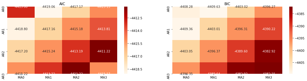
로그리듬값의 최적의 1차계 매개 변수 조합은 (0,1,1) 이므로 간단하고 간단하다. 로그_리턴 (로그리듬률) 은 동일한 연산을 수행한다. AIC 최적 값은 (4,3), BIC 최적 값은 (0,1) 이다. 따라서 로그_리턴 (로그리듬률) 의 최적의 매개 변수 조합은 (0,1) 이다.

4-2 ARMA 모델링 및 매칭

분기 계수는 필요하지 않지만 SARIMAX는 특성이 더 풍부하므로 모델링을 위해이 모델을 선택하고 다음과 같이 설명적 분석을 결정했습니다.

[11]에서:

params = (0, 0, 1)
training_model = smt.SARIMAX(endog=kline_all['log_return'], trend='c', order=params, seasonal_order=(0, 0, 0, 0))
model_results = training_model.fit(disp=False)
model_results.summary()

아웃[11]: 국가 공간 모델 결과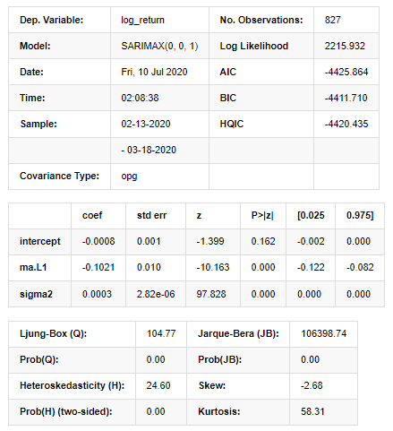

경고: [1] 그라디언트의 외부 곱 (복합 단계) 을 사용하여 계산된 코바리언스 행렬. [27]에서:

model_results.plot_diagnostics(figsize=(18, 10));

외출 [1]:

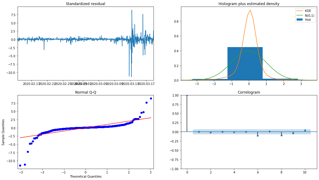
히스토그램의 확률 밀도 KDE는 정상적인 분포 N (0,1) 에서 멀리 떨어져 있으며, 잔액이 정상적인 분포가 아니라는 것을 나타냅니다. QQ 퀀틸 그래프에서 표준 정상 분포에서 표본 샘플의 잔액은 선형 추세를 완전히 따르지 않으므로 잔액이 정상적인 분포가 아니며 백색 노이즈에 가깝다는 것이 다시 확인됩니다.

그런 다음, 그 모델이 사용될 수 있는지 여부는 여전히 테스트되어야합니다.

4-3. 모델 테스트

잔액의 일치 효과는 이상적이지 않으므로 데르빈 왓슨 테스트를 수행했습니다. 테스트의 원래 가설은 순서가 자가 상관관계가 없으며 대체 가설 순서가 고정되어 있다는 것입니다. 또한, LB, JB 및 H 테스트의 P 값이 0.05% 신뢰 수준의 결정적 값보다 작으면 원래 가설이 거부됩니다.

[12]에서:

het_method='breakvar'
norm_method='jarquebera'
sercor_method='ljungbox'

(het_stat, het_p) = model_results.test_heteroskedasticity(het_method)[0]
norm_stat, norm_p, skew, kurtosis = model_results.test_normality(norm_method)[0]

sercor_stat, sercor_p = model_results.test_serial_correlation(method=sercor_method)[0]
sercor_stat = sercor_stat[-1] # The last value of the maximum period
sercor_p = sercor_p[-1]

dw = sm.stats.stattools.durbin_watson(model_results.filter_results.standardized_forecasts_error[0, model_results.loglikelihood_burn:])

arroots_outside_unit_circle = np.all(np.abs(model_results.arroots) > 1)
maroots_outside_unit_circle = np.all(np.abs(model_results.maroots) > 1)

print('Test heteroskedasticity of residuals ({}): stat={:.3f}, p={:.3f}'.format(het_method, het_stat, het_p));
print('\nTest normality of residuals ({}): stat={:.3f}, p={:.3f}'.format(norm_method, norm_stat, norm_p));
print('\nTest serial correlation of residuals ({}): stat={:.3f}, p={:.3f}'.format(sercor_method, sercor_stat, sercor_p));
print('\nDurbin-Watson test on residuals: d={:.2f}\n\t(NB: 2 means no serial correlation, 0=pos, 4=neg)'.format(dw))
print('\nTest for all AR roots outside unit circle (>1): {}'.format(arroots_outside_unit_circle))
print('\nTest for all MA roots outside unit circle (>1): {}'.format(maroots_outside_unit_circle))

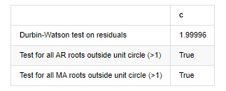
root_test=pd.DataFrame(index=['Durbin-Watson test on residuals','Test for all AR roots outside unit circle (>1)','Test for all MA roots outside unit circle (>1)'],columns=['c'])
root_test['c']['Durbin-Watson test on residuals']=dw
root_test['c']['Test for all AR roots outside unit circle (>1)']=arroots_outside_unit_circle
root_test['c']['Test for all MA roots outside unit circle (>1)']=maroots_outside_unit_circle
root_test

아웃[12]: 잔류의 heteroskedasticity 테스트 (breakvar): stat=24.598, p=0.000

잔류물 (jarquebera) 의 검사 정상성: stat=106398.739, p=0.000

잔류물질의 테스트 일련 상관관계 (ljungbox): stat=104.767, p=0.000

잔류에 대한 더빈-왓슨 테스트: d=2.00 2는 연쇄 상관관계가 없다는 뜻입니다. 0=pos, 4=neg)

단위 원 (>1) 외의 모든 AR 뿌리에 대한 테스트: 사실

단위 원 바깥의 모든 MA 뿌리에 대한 테스트 (>1): 사실

[13]에서:

kline_all['log_price_dif1'] = kline_all['log_price'].diff(1)
kline_all = kline_all[1:]
kline_train = kline_all

training_label = 'log_return'
training_ts = pd.DataFrame(kline_train[training_label], dtype=np.float)

delta = model_results.fittedvalues - training_ts[training_label]
adjR = 1 - delta.var()/training_ts[training_label].var()
adjR_test=pd.DataFrame(index=['adjR2'],columns=['Value'])
adjR_test['Value']['adjR2']=adjR**2
adjR_test

아웃[13]:

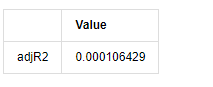
더빈 왓슨 테스트 통계는 2에 해당하는 경우, 일련에 상관관계가 없으며, 그 통계 값은 (0,4) 사이에 분포된다는 것을 확인합니다. 0에 가깝다는 것은 긍정적 상관관계가 높다는 것을 의미하며, 4에 가깝다는 것은 부정적인 상관관계가 높다는 것을 의미합니다. 여기서는 대략 2에 해당합니다. 다른 테스트의 P 값은 충분히 작고, 단위 특성 뿌리는 단위 원 밖에서 있으며, 수정된 adjR2의 값이 클수록 더 좋습니다. 측정의 전반적인 결과는 만족스럽지 않습니다.

[14]에서:

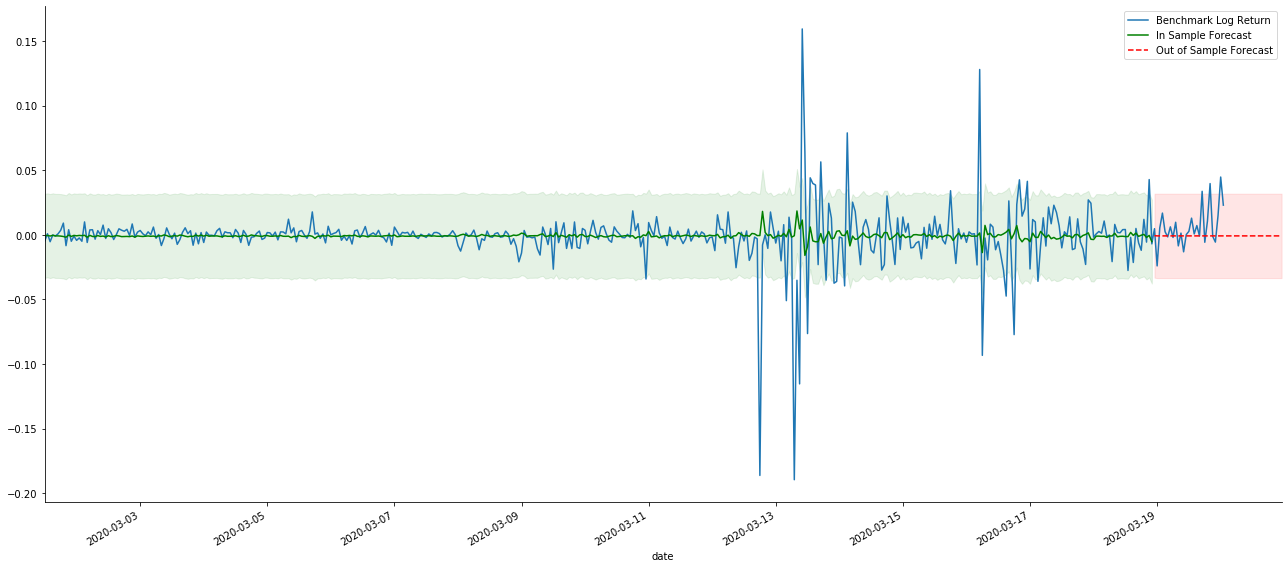
model_results.params

아웃[14]: 가로막는 -0.000817 ma.L1 -0.102102 시그마2 0.000275 d 타입: float64

요약하자면, 이 순서 설정 매개 변수는 기본적으로 시간 계열 모델링 및 후속 변동성 모델링의 요구 사항을 충족시킬 수 있지만 매칭 효과는 다음과 같습니다. 모델 표현은 다음과 같습니다.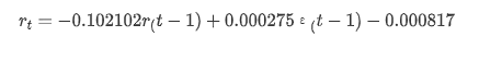

4-4. 모델 예측

다음으로, 훈련된 모델은 앞으로 매칭됩니다. statsmodels는 매칭 및 예측을 위해 정적 및 동적 옵션을 제공합니다. 차이점은 관측 값이 예측의 다음 단계에 사용되거나 이전 단계에서 생성된 예측 값이 반복적으로 사용되는지에 있습니다. log_return (소수의 로그리듬 비율) 의 예측 효과는 다음과 같습니다.

[37]에서:

start_date = '2020-02-28 12:00:00+08:00'
end_date = start_date 

pred_dy = model_results.get_prediction(start=start_date, dynamic=False)
pred_dy_ci = pred_dy.conf_int()

fig, ax = plt.subplots(nrows=1, ncols=1, figsize=(18, 6))
ax.plot(kline_all['log_return'].loc[start_date:], label='Log Return', linestyle='-')
ax.plot(pred_dy.predicted_mean.loc[start_date:], label='Forecast Log Return', linestyle='--')
ax.fill_between(pred_dy_ci.index,pred_dy_ci.iloc[:, 0],pred_dy_ci.iloc[:, 1], color='g', alpha=.25)

plt.ylabel("BTC Log Return")
plt.legend(loc='best')
plt.tight_layout()
sns.despine()

아웃[37]:

정적 모드의 샘플에 대한 적합 효과는 훌륭하며, 샘플 데이터는 거의 95% 신뢰도 간격으로 커버 될 수 있으며, 동적 모드는 약간 통제되지 않습니다.

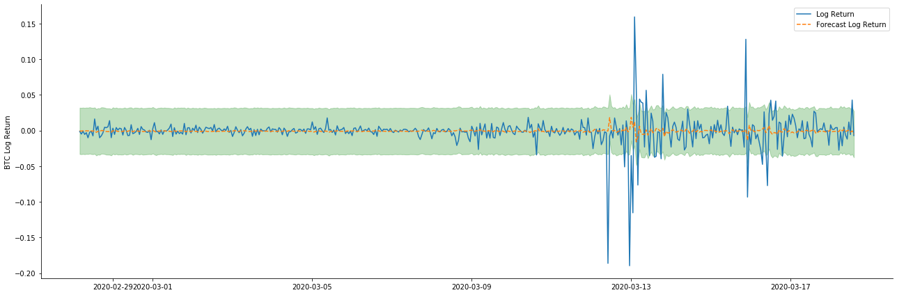
그래서 동적 모드에서 데이터 일치 효과를 살펴봅시다:

[38]에서:

start_date = '2020-02-28 12:00:00+08:00'
end_date = start_date 

pred_dy = model_results.get_prediction(start=start_date, dynamic=True)
pred_dy_ci = pred_dy.conf_int()

fig, ax = plt.subplots(nrows=1, ncols=1, figsize=(18, 6))
ax.plot(kline_all['log_return'].loc[start_date:], label='Log Return', linestyle='-')
ax.plot(pred_dy.predicted_mean.loc[start_date:], label='Forecast Log Return', linestyle='--')
ax.fill_between(pred_dy_ci.index,pred_dy_ci.iloc[:, 0],pred_dy_ci.iloc[:, 1], color='g', alpha=.25)

plt.ylabel("BTC Log Return")
plt.legend(loc='best')
plt.tight_layout()
sns.despine()

아웃[38]:

두 모델의 샘플에 대한 적합 효과는 훌륭하고 평균 값은 95% 신뢰 간격에 거의 커버 될 수 있지만 정적 모델은 분명히 더 적합하다는 것을 알 수 있습니다. 다음으로 50 단계의 예측 효과를 살펴 보겠습니다.

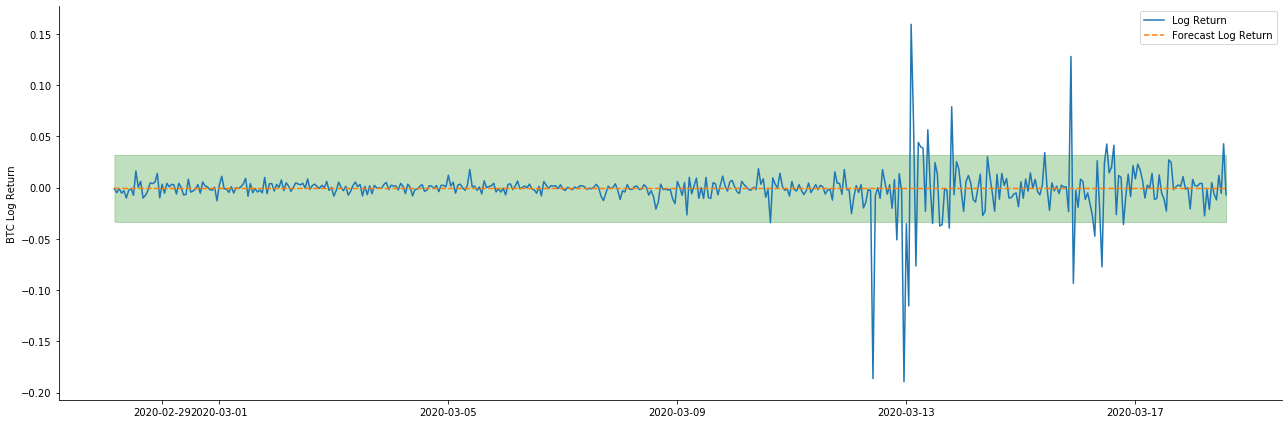
[41]에서:

# Out-of-sample predicted data predict()
start_date = '2020-03-01 12:00:00+08:00'
end_date = '2020-03-20 23:00:00+08:00'
model = False

predict_step = 50
predicts_ARIMA_normal = model_results.get_prediction(start=start_date, dynamic=model, full_reports=True)
ci_normal = predicts_ARIMA_normal.conf_int().loc[start_date:]

predicts_ARIMA_normal_out = model_results.get_forecast(steps=predict_step, dynamic=model)
ci_normal_out = predicts_ARIMA_normal_out.conf_int().loc[start_date:end_date]

fig, ax = plt.subplots(figsize=(18,8))
kline_test.loc[start_date:end_date, 'log_return'].plot(ax=ax, label='Benchmark Log Return')

predicts_ARIMA_normal.predicted_mean.plot(ax=ax, style='g', label='In Sample Forecast')
ax.fill_between(ci_normal.index, ci_normal.iloc[:,0], ci_normal.iloc[:,1], color='g', alpha=0.1)

predicts_ARIMA_normal_out.predicted_mean.loc[:end_date].plot(ax=ax, style='r--', label='Out of Sample Forecast')
ax.fill_between(ci_normal_out.index, ci_normal_out.iloc[:,0], ci_normal_out.iloc[:,1], color='r', alpha=0.1)

plt.tight_layout()
plt.legend(loc='best')
sns.despine()

아웃[41]:

표본 내의 데이터의 일치는 앞으로의 예측이기 때문에 표본 내의 정보의 양이 충분하면 정적 모델은 과도한 일치에 취약하며, 동적 모델은 신뢰할 수있는 종속 변수가 없으며 반복 후 효과는 점점 악화됩니다. 표본 외부의 데이터를 예측할 때 모델은 표본 내의 동적 모델과 동등하므로 장기 예측의 오류 용어의 정확도는 낮을 것입니다.

만약 우리가 수익률 예측을 로그_프라이스 (로그아리듬 가격) 로 역전하면, 일치는 아래 그림에서 나타납니다.

[42]에서:

params = (0, 1, 1)
mod = smt.SARIMAX(endog=kline_all['log_price'], trend='c', order=params, seasonal_order=(0, 0, 0, 0))
res = mod.fit(disp=False)

start_date = '2020-03-01 12:00:00+08:00'
end_date = '2020-03-15 23:00:00+08:00'

predicts_ARIMA_normal = res.get_prediction(start=start_date, dynamic=False, full_results=False)
predicts_ARIMA_dynamic = res.get_prediction(start=start_date, dynamic=True, full_results=False)

fig, ax = plt.subplots(figsize=(18,6))
kline_test.loc[start_date:end_date, 'log_price'].plot(ax=ax, label='Log Price')

predicts_ARIMA_normal.predicted_mean.loc[start_date:end_date].plot(ax=ax, style='r--', label='Normal Prediction')
ci_normal = predicts_ARIMA_normal.conf_int().loc[start_date:end_date]
ax.fill_between(ci_normal.index, ci_normal.iloc[:,0], ci_normal.iloc[:,1], color='r', alpha=0.1)

predicts_ARIMA_dynamic.predicted_mean.loc[start_date:end_date].plot(ax=ax, style='g', label='Dynamic Prediction')
ci_dynamic = predicts_ARIMA_dynamic.conf_int().loc[start_date:end_date]
ax.fill_between(ci_dynamic.index, ci_dynamic.iloc[:,0], ci_dynamic.iloc[:,1], color='g', alpha=0.1)

plt.tight_layout()
plt.legend(loc='best')
sns.despine()

아웃[42]:

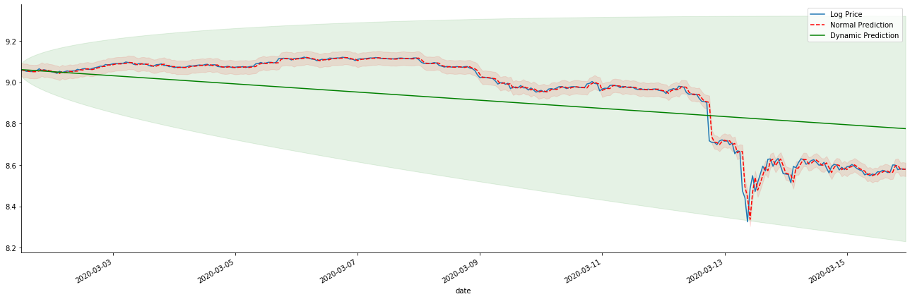
정적 모형의 일치 장점과 동적 모형과 정적 모형의 극심한 차이점을 장기 예측에서 쉽게 볼 수 있습니다. 빨간 점점 선과 분홍색 범위... 당신은이 모델의 예측이 잘못되었다고 말할 수 없습니다. 결국, 그것은 이동 평균의 경향을 완전히 포함하지만... 그것은 의미가 있습니까?

사실 ARMA 모델 자체는 틀린 것이 아닙니다. 왜냐하면 문제는 모델 자체가 아니라 사물의 객관적 논리이기 때문입니다. 시간 계열 모델은 이전과 후속 관측 사이의 상관관계에 따라만 확립 될 수 있습니다. 따라서 백색 노이즈 시리즈를 모델링하는 것은 불가능합니다. 따라서 이전 모든 작업은 BTC의 수익률 시리즈가 독립적이고 동일하게 분포할 수 없다는 대담한 가정에 기반합니다.

일반적으로 수익률 시리즈는 마르틴게일 차이 시리즈이며, 이는 수익률이 예측 불가능하며 해당 시장의 약한 효율성 가정이 유효하다는 것을 의미합니다. 개별 샘플의 수익률이 일정 수준의 자가 상관관계를 가지고 있다고 가정했으며 동일한 분포 가정은 또한 훈련 세트에 적용 가능한 매칭 모델을 만들기 위해 간단한 ARMA 모델을 매칭 할 수 있으므로 예측 효과가 좋지 않을 것입니다.

그러나 일치된 잔류 순서는 마틴게일 차이 순서이기도 하다. 마틴게일 차이 순서는 독립적이고 동일하게 분포되지 않을 수 있지만 조건적 변동은 과거의 값에 의존할 수 있으므로 1차 자동 상관관계가 사라졌지만 여전히 높은 순위의 자동 상관관계가 있으며 이는 또한 변동성을 모델링하고 관찰하는 중요한 전제 조건이다.

이러한 논리가 유효하다면, 다양한 변동성 모델을 구축하는 전제 또한 유효합니다. 따라서 수익률 시리즈에 대해, 효율성이 약한 시장이 만족되면 평균 값은 예측하기가 어렵지만 변동은 예측 가능합니다. 그리고 매칭된 ARMA는 공정한 품질의 시간 시리즈 벤치마크를 제공하므로 품질은 변동성 예측의 품질을 결정합니다.

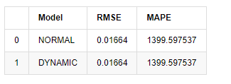
마지막으로, 예측의 효과를 간단하게 평가해보겠습니다. 평가 기준으로 오류를 사용하면 표본 내부와 외부의 지표는 다음과 같습니다.

[15]에서:

start = '2020-02-14 00:00:00+08:00'
predicts_ARIMA_normal = model_results.get_prediction(dynamic=False)
predicts_ARIMA_dynamic = model_results.get_prediction(dynamic=True)
training_label = 'log_return'

compare_ARCH_X = pd.DataFrame()
compare_ARCH_X['Model'] = ['NORMAL','DYNAMIC']
compare_ARCH_X['RMSE'] = [rmse(predicts_ARIMA_normal.predicted_mean[1:], kline_test[training_label][:826]),
                          rmse(predicts_ARIMA_dynamic.predicted_mean[1:], kline_test[training_label][:826])]
compare_ARCH_X['MAPE'] = [mape(predicts_ARIMA_normal.predicted_mean[:50], kline_test[training_label][:50]),
                          mape(predicts_ARIMA_dynamic.predicted_mean[:50], kline_test[training_label][:50])]
compare_ARCH_X

외출[15]: 루트 평균 제곱 오류 (RMSE): 0.0184 루트 평균 제곱 오류 (RMSE): 0.0167 평균 절대 비율 오류 (MAPE): 2.25e+03 평균 절대 비율 오류 (MAPE): 395

정적 모델은 예측 값과 실제 값 사이의 오류 일치 측면에서 동적 모델보다 약간 낫다는 것을 알 수 있습니다. 그것은 기본적으로 기대에 부합하는 비트코인의 로그아리듬적 수익률과 잘 일치합니다. 동적 예측은 더 정확한 변수 정보가 부족하며 오류는 반복으로 확대되므로 예측 효과는 약합니다. MAPE는 100% 이상이기 때문에 두 모델의 실제 매칭 품질은 이상적이지 않습니다.

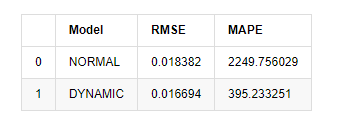
[18]에서:

predict_step = 50
predicts_ARIMA_normal_out = model_results.get_forecast(steps=predict_step, dynamic=False)
predicts_ARIMA_dynamic_out = model_results.get_forecast(steps=predict_step, dynamic=True)
testing_ts = kline_test
training_label = 'log_return'

compare_ARCH_X = pd.DataFrame()
compare_ARCH_X['Model'] = ['NORMAL','DYNAMIC']
compare_ARCH_X['RMSE'] = [get_rmse(predicts_ARIMA_normal_out.predicted_mean, testing_ts[training_label]),
                          get_rmse(predicts_ARIMA_dynamic_out.predicted_mean, testing_ts[training_label])]
compare_ARCH_X['MAPE'] = [get_mape(predicts_ARIMA_normal_out.predicted_mean, testing_ts[training_label]),
                          get_mape(predicts_ARIMA_dynamic_out.predicted_mean, testing_ts[training_label])]
compare_ARCH_X

아웃[18]:

표본 외부의 다음 예측은 이전 단계의 결과에 의존하기 때문에 동적 모델만이 효과적입니다. 그러나 동적 모델의 장기 오류 결함은 전체 모델의 예측 능력이 충분하지 않기 때문에 다음 단계가 예측됩니다.

요약하자면, ARMA 모델 정적 모델은 비트코인의 샘플 내 수익률을 맞추기 위해 적합합니다. 수익률의 단기 예측은 신뢰 간격을 효과적으로 커버 할 수 있지만 장기 예측은 매우 어렵습니다. 이는 시장의 약한 효과를 충족시킵니다. 테스트 후 샘플 간격 내의 수익률은 후속 변동성 관찰의 전제를 충족시킵니다.

5. ARCH 효과

ARCH 모델 효과는 조건적 이성분열성 염기서열의 일련 상관관계이다. 혼합 테스트 Ljung Box는 ARCH 효과가 있는지 여부를 결정하기 위해 잔류 제곱 일련의 상관관계를 테스트하는 데 사용됩니다. ARCH 효과 테스트가 통과되면, 즉 시리즈가 이성분열성을 가지고 있다면, 평균 방정식과 변동성 방정식을 공동으로 추정하기 위해 GARCH 모델링의 다음 단계를 수행 할 수 있습니다. 그렇지 않으면 모델을 최적화하고 재조정해야합니다.

여기 몇 개의 데이터 세트와 글로벌 변수를 준비했습니다.

[33]에서:

count_num = 100000
start_date = '2020-03-01'

df = get_bars('huobi.btc_usdt', '1m', count=count_num, start=start_date)  # Take the minute data
kline_1m = pd.DataFrame(df['close'], dtype=np.float)
kline_1m.index.name = 'date'
kline_1m['log_price'] = np.log(kline_1m['close'])
kline_1m['return'] = kline_1m['close'].pct_change().dropna()
kline_1m['log_return'] = kline_1m['log_price'] - kline_1m['log_price'].shift(1)

kline_1m['squared_log_return'] = np.power(kline_1m['log_return'], 2)

kline_1m['return_100x'] = np.multiply(kline_1m['return'], 100)
kline_1m['log_return_100x'] = np.multiply(kline_1m['log_return'], 100)  # Enlarge 100 times

df = get_bars('huobi.btc_usdt', '1h', count=count_num, start=start_date)  # Take the hour data
kline_test = pd.DataFrame(df['close'], dtype=np.float)
kline_test.index.name = 'date'
kline_test['log_price'] = np.log(kline_test['close'])  # Calculate the daily logarithmic rate of return
kline_test['return'] = kline_test['log_price'].pct_change().dropna()
kline_test['log_return'] = kline_test['log_price'] - kline_test['log_price'].shift(1)  # Calculate the logarithmic rate of return
kline_test['squared_log_return'] = np.power(kline_test['log_return'], 2)  # Exponential square of log daily return rate

kline_test['return_100x'] = np.multiply(kline_test['return'], 100)
kline_test['log_return_100x'] = np.multiply(kline_test['log_return'], 100)  # Enlarge 100 times

kline_test['realized_variance_1_hour'] = kline_1m.loc[:, 'squared_log_return'].resample('h', closed='left', label='left').sum().copy() # Resampling to days 
kline_test['realized_volatility_1_hour'] = np.sqrt(kline_test['realized_variance_1_hour'])  # Volatility of variance derivation

kline_test = kline_test[4:-2500]
kline_test.head(3)

아웃[33]:

[22]에서:

cc = 3
model_p = 1
predict_lag = 30
label = 'log_return'

training_label = label
training_ts = pd.DataFrame(kline_test[training_label], dtype=np.float)

training_arch_label = label
training_arch = pd.DataFrame(kline_test[training_arch_label], dtype=np.float)

training_garch_label = label
training_garch = pd.DataFrame(kline_test[training_garch_label], dtype=np.float)

training_egarch_label = label
training_egarch = pd.DataFrame(kline_test[training_egarch_label], dtype=np.float)

training_arch.plot(figsize = (18,4))

외출[22]:

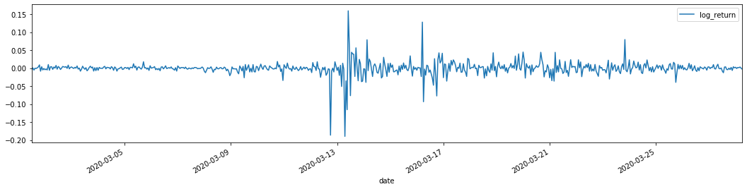
로그아리듬 반환률은 위에 표시되어 있습니다. 다음으로, 우리는 샘플의 ARCH 효과를 테스트해야합니다. 우리는 ARMA를 기반으로 샘플 내에서 잔류 시리즈를 설정합니다. 일부 시리즈와 잔류 및 잔류의 제곱 시리즈는 먼저 계산됩니다.

[20]에서:

training_arma_model = smt.SARIMAX(endog=training_ts, trend='c', order=(0, 0, 1), seasonal_order=(0, 0, 0, 0))
arma_model_results = training_arma_model.fit(disp=False)
arma_model_results.summary()
training_arma_fitvalue = pd.DataFrame(arma_model_results.fittedvalues,dtype=np.float)
at = pd.merge(training_ts, training_arma_fitvalue, on='date')
at.columns = ['log_return', 'model_fit']
at['res'] = at['log_return'] - at['model_fit']
at['res2'] = np.square(at['res'])
at.head()

외출[20]:

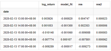
그 다음 샘플의 잔류 시리즈는 그래프로 표시됩니다.

[69]에서:

fig, ax = plt.subplots(figsize=(18, 6))
ax1 = fig.add_subplot(2,1,1)
at['res'][1:].plot(ax=ax1,label='resid')
plt.legend(loc='best')

ax2 = fig.add_subplot(2,1,2)
at['res2'][1:].plot(ax=ax2,label='resid2')

plt.legend(loc='best')
plt.tight_layout()
sns.despine()

아웃[69]:

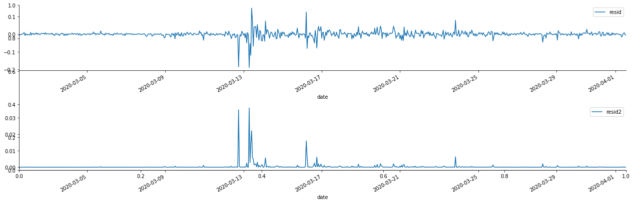
잔류열이 명백한 집적 특성을 가지고 있음을 볼 수 있으며, 일련이 ARCH 효과를 가지고 있다고 처음에는 판단 할 수 있습니다. ACF는 또한 제곱 잔류수의 자율 상관관계를 테스트하기 위해 사용되며 결과는 다음과 같습니다.

[70]에서:

figure = plt.figure(figsize=(18,4))
ax1 = figure.add_subplot(111)
fig = sm.graphics.tsa.plot_acf(at['res2'],lags = 40, ax=ax1)

아웃[70]:

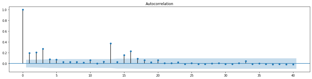
시리즈 혼합 테스트의 원래 가정은 시리즈가 상관관계가 없다는 것입니다. 첫 20 개의 데이터 순서의 대응 P 값이 0.05% 신뢰 수준의 결정적 값보다 작다는 것을 볼 수 있습니다. 따라서 원래 가정은 거부됩니다. 즉, 시리즈의 잔류는 ARCH 효과를 가지고 있습니다. 변동 모형은 잔류 시리즈의 이성분열성에 맞게 ARCH 타입 모형을 통해 설정 할 수 있으며 더 나아가 변동성을 예측 할 수 있습니다.

6. GARCH 모델링

GARCH 모델링을 수행하기 전에, 우리는 일련의 뚱뚱한 꼬리 부분을 다루어야 합니다. 가설에 있는 일련의 오류 용어는 정상 분포 또는 t 분포에 적합해야 하기 때문에, 그리고 우리는 이전에 양산 시리즈가 뚱뚱한 꼬리 분포를 가지고 있다는 것을 검증했기 때문에, 우리는 이 부분을 설명하고 보완해야 합니다.

GARCH 모델링에서 오류 항목은 정상 분포, t 분포, GED (일반 오류 분포) 분포 및 skewed 학생 t 분포의 옵션을 제공합니다. AIC 기준에 따라 우리는 모든 옵션의 결과를 비교하고 G의 최고의 매칭 정도를 얻기 위해 집계 합동 회귀 추정치를 사용합니다.

관련

더 많은