成熟的分类器：SVM是一个强大且成熟的二元（或多元）分类算法。预测“涨”还是“跌”正好是一个典型的二元分类问题。 非线性能力：通过使用核函数（如RBF核），SVM可以捕捉到输入特征之间复杂的非线性关系，这对于金融市场数据至关重要。 特征驱动：模型的效果很大程度上取决于你喂给它的“特征”（Features）。现在计算的alpha因子就是一个很好的开始，我们可以构建更多这样的特征来提升预测能力。 这次我最开始用到了3个特征大纲： 1：高频订单流特征： alpha_1min: 基于过去1分钟所有tick计算出的订单流不平衡因子。 alpha_5min: 基于过去5分钟所有tick计算出的订单流不平衡因子。 alpha_15min: 基于过去15分钟所有tick计算出的订单流不平衡因子。 ofi_1min (Order Flow Imbalance): 1分钟内，（买入成交量 / 卖出成交量）的比率。这个比alpha更直接。 vol_per_trade_1min: 1分钟内，平均每笔交易的成交量。大单冲击市场的迹象。

2：价格与波动率特征： log_return_5min: 过去5分钟的对数收益率 log(Pt / P{t-5min})。 volatility_15min: 过去15分钟对数收益率的标准差，衡量短期波动性。 atr_14 (Average True Range): 基于过去14根1分钟K线的ATR值，经典的波动率指标。 rsi_14 (Relative Strength Index): 基于过去14根1分钟K线的RSI值，衡量超买超卖。

3：时间特征： hour_of_day: 当前小时数 (0-23)。市场在不同时间段有不同表现（如亚洲/欧洲/美洲时段）。 day_of_week: 周几 (0-6)。周末和工作日的波动模式不同。

def calculate_features_and_labels(klines):
    """
    核心函数
    """
    features = []
    labels = []
    
    # 为了计算RSI等指标，我们需要价格序列
    close_prices = [k['close'] for k in klines]
    
    # 从第30根K线开始，因为需要足够的前置数据
    for i in range(30, len(klines) - PREDICT_HORIZON):
        # 1. 价格与波动率特征
        price_change_15m = (klines[i]['close'] - klines[i-15]['close']) / klines[i-15]['close']
        volatility_30m = np.std(close_prices[i-30:i])
        
        # 计算RSI
        diffs = np.diff(close_prices[i-14:i+1])
        gains = np.sum(diffs[diffs > 0]) / 14
        losses = -np.sum(diffs[diffs < 0]) / 14
        rs = gains / (losses + 1e-10)
        rsi_14 = 100 - (100 / (1 + rs))
        
        # 2. 时间特征
        dt_object = datetime.fromtimestamp(klines[i]['ts'] / 1000)
        hour_of_day = dt_object.hour
        day_of_week = dt_object.weekday()
        
        # 组合所有特征
        current_features = [price_change_15m, volatility_30m, rsi_14, hour_of_day, day_of_week]
        features.append(current_features)
        
        # 3. 数据标注
        future_price = klines[i + PREDICT_HORIZON]['close']
        current_price = klines[i]['close']
        
        if future_price > current_price * (1 + SPREAD_THRESHOLD):
            labels.append(0) # 涨
        elif future_price < current_price * (1 - SPREAD_THRESHOLD):
            labels.append(1) # 跌
        else:
            labels.append(2) # 横盘

然后用三分类去区分 涨 跌 横盘。

筛选特征筛选的核心思想：寻找“神队友”，剔除“猪队友”

我们的目标是找到这样一组特征： * 高相关性 (High Relevance)：每个特征都与未来的价格变动（我们的目标标签）有较强的关联。 * 低冗余性 (Low Redundancy): 特征之间不要包含太多重复信息。例如，“5分钟动量”和“6分钟动量”高度相似，放两个进去对模型提升不大，反而可能引入噪音。 * 稳定性 (Stability): 特征的有效性不能随时间变化太快。一个只在某一天有效的特征是危险的。

def run_analysis_report(X, y, clf, scaler):
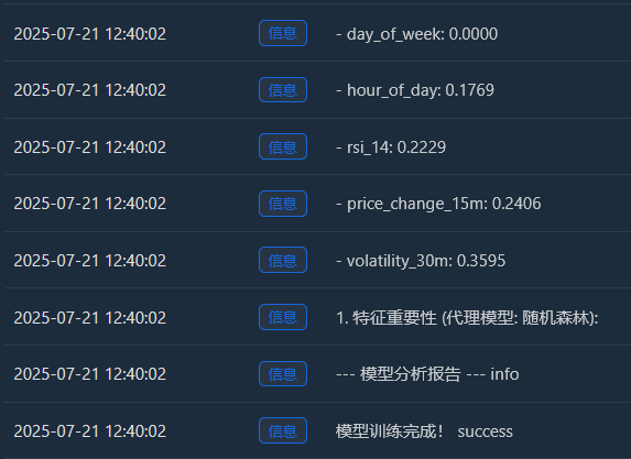
    Log("--- 模型分析报告 ---", "info")
    Log("1. 特征重要性 (代理模型: 随机森林):")
    rf = RandomForestClassifier(n_estimators=50, random_state=42); rf.fit(X, y)
    importances = sorted(zip(g_feature_names, rf.feature_importances_), key=lambda x: x[1], reverse=True)
    for name, importance in importances: Log(f"   - {name}: {importance:.4f}")
    Log("2. 特征与标签的互信息:"); mi_scores = mutual_info_classif(X, y)
    mi_scores = sorted(zip(g_feature_names, mi_scores), key=lambda x: x[1], reverse=True)
    for name, score in mi_scores: Log(f"   - {name}: {score:.4f}")
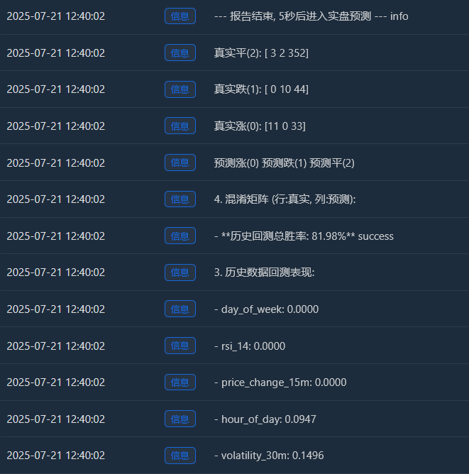
    Log("3. 历史数据回测表现:"); y_pred = clf.predict(scaler.transform(X)); accuracy = accuracy_score(y, y_pred)
    Log(f"   - **历史回测总胜率: {accuracy * 100:.2f}%**", "success")
    Log("4. 混淆矩阵 (行:真实, 列:预测):"); cm = confusion_matrix(y, y_pred)
    Log("      预测涨(0) 预测跌(1) 预测平(2)"); Log(f"真实涨(0): {cm[0] if len(cm) > 0 else [0,0,0]}")
    Log(f"真实跌(1): {cm[1] if len(cm) > 1 else [0,0,0]}"); Log(f"真实平(2): {cm[2] if len(cm) > 2 else [0,0,0]}")
    profit_chart = Chart({'title': {'text': f'历史回测净值曲线 (胜率: {accuracy*100:.2f}%)'}}); profit_chart.reset(); balance = 1
    for i in range(len(y)):
        if y_pred[i] == y[i] and y[i] != 2: balance *= (1 + 0.01)
        elif y_pred[i] != y[i] and y_pred[i] != 2: balance *= (1 - 0.01)
        profit_chart.add(i, balance)
    Log("--- 报告结束, 5秒后进入实盘预测 ---", "info"); Sleep(5000)

流程是： 收集数据 特征重要性 特征与标签的互信息和回测信息

我本来想着能弄一个65%的胜率就可以了，但是没想到到达了81.98% 我的第一反应应该是：“太棒了，但也太好了，好得有点不真实。这里面一定有值得深究的地方。”

1. 深入解读分析报告，逐一解读报告内容：

1. 特征重要性 & 互信息: volatility_30m (波动率) 和 price_change_15m (价格变化) 成为了最重要的特征。这非常符合逻辑，说明市场的近期趋势和波动状态是预测未来的最强依据。 hour_of_day (小时) 也有一定的贡献，说明模型捕捉到了一天内不同时段的交易模式。 rsi_14 和 day_of_week (星期) 的贡献度几乎为0，这提示我们，在当前的数据集和特征组合下，这两个特征可能是“猪队友”，未来可以考虑移除它们以简化模型，防止噪音。
2. 混淆矩阵 (这部分信息量巨大！) 真实涨(0): [11 0 33] -> 在44次（11+0+33）真实上涨中，模型正确预测了11次，但有33次把它预测成了“盘整”。 真实跌(1): [ 0 10 44] -> 在54次（0+10+44）真实下跌中，模型正确预测了10次，但有44次把它预测成了“盘整”。 真实平(2): [ 3 2 352] -> 在357次（3+2+352）真实盘整中，模型正确预测了352次！
3. 历史回测总胜率: 81.98% 这个高胜率的核心来源，是模型在预测“盘整”时极高的准确率！ 在总共约455个样本中，有超过350个都是盘整市，而模型几乎完美地识别了它们。 这本身是一个非常有价值的能力！一个能准确告诉你“现在最好别动”的模型，可以帮你省下大量的手续费和无效交易。

2 为什么实盘胜率可能会低于81.98%？

1. “盘整”的定义过于宽松: 我们的SPREAD_THRESHOLD是0.5%。在15分钟内，价格波动不超过0.5%是非常常见的。这导致了我们的数据集中，“盘整”样本占了绝大多数（约80%）。模型很“聪明”地学会了：“当我没把握时，猜‘盘整’就对了，准确率很高。” 这在统计上是正确的，但在交易上，我们更关心的是对涨跌的预测能力。
2. 对涨跌的预测能力: 预测上涨的胜率: 模型预测了 11 + 0 + 3 = 14 次上涨，其中只有11次是正确的。胜率是 11 / 14 = 78.5%。非常棒！ 预测下跌的胜率: 模型预测了 0 + 10 + 2 = 12 次下跌，其中有10次是正确的。胜率是 10 / 12 = 83.3%。同样非常出色！
3. 样本内过拟合 (In-Sample Overfitting): 这个测试是在模型“已知”的数据上进行的（即用这些数据训练，再用它们来测试）。这就像让一个学生做他刚刚做过的原题，分数通常会很高。模型在未知的、全新的数据上（实盘）的表现，几乎总会比这个分数要低。

现在拥有了一个初步的、但潜力巨大的“Alpha模型”。81.98% 这个数字，虽然我们不能直接把它当作未来的实盘预期，但它是一个强烈的积极信号，证明了数据中确实存在可预测的规律，而且我们的框架成功地捕捉到了它！ 我们现在的感觉，就像是在一座金山的山脚下，挖到了第一块成色极高的金矿石。接下来，我们要做的不是马上把它卖掉，而是要通过更专业的工具和技术（优化特征、调整参数），把整座金山更高效、更稳定地挖掘出来。

现在引入“微观世界”的战争迷雾——订单流与订单簿特征 第一步：升级数据采集——订阅更深的频道 要获取订单簿数据，必须修改WebSocket的连接方式，从只订阅aggTrade（成交）升级为同时订阅aggTrade和depth（深度）。 这需要我们使用一种更通用的多流订阅（Multi-Stream）URL。 第二步：升级特征工程——构建“海陆空”三位一体的特征矩阵 我们将在calculate_features_and_labels函数中，增加以下全新的特征：

1. 订单流特征 (Alpha - 空军): alpha_15m: 15分钟的订单流不平衡因子。这是我们之前讨论过的核心订单流指标。
2. 订单簿特征 (Book - 陆军): wobi_10s: 过去10秒的加权订单簿不平衡性 (Weighted Order Book Imbalance)。这是一个非常高频的、衡量盘口买卖压力的指标。 spread_10s: 过去10秒的平均买一卖一价差。反映短期流动性。
3. 原有特征 (Price - 海军): 我们将保留上一版中表现最好的特征，并进行优化。

这个新的特征矩阵，就像一个联合作战司令部，同时掌握了来自“海（价格趋势）”、“陆（盘口阵地）”、“空（成交冲击）”三方的实时情报，决策能力将远超从前。 代码如下：

import json
import math
import time
import websocket
import threading
from datetime import datetime
import numpy as np
from sklearn import svm
from sklearn.preprocessing import StandardScaler
from sklearn.metrics import confusion_matrix, accuracy_score
from sklearn.feature_selection import mutual_info_classif
from sklearn.ensemble import RandomForestClassifier

# ========== 全局配置 ==========
TRAIN_BARS = 100
PREDICT_HORIZON = 15
SPREAD_THRESHOLD = 0.005
SYMBOL_FMZ = "ETH_USDT" 
SYMBOL_API = SYMBOL_FMZ.replace('_', '').lower()
WEBSOCKET_URL = f"wss://fstream.binance.com/stream?streams={SYMBOL_API}@aggTrade/{SYMBOL_API}@depth20@100ms"

# ========== 全局状态变量 ==========
g_model, g_scaler = None, None
g_klines_1min, g_ticks, g_order_book_history = [], [], []
g_last_kline_ts = 0
g_feature_names = ['price_change_15m', 'volatility_30m', 'rsi_14', 'hour_of_day', 
                   'alpha_15m', 'wobi_10s', 'spread_10s']

# ========== 特征工程与模型训练 ==========
def calculate_features_and_labels(klines, ticks, order_books_history, is_realtime=False):
    features, labels = [], []
    close_prices = [k['close'] for k in klines]
    
    # 根据是训练还是实时预测，决定循环范围
    start_index = 30
    end_index = len(klines) - PREDICT_HORIZON if not is_realtime else len(klines)

    for i in range(start_index, end_index):
        kline_start_ts = klines[i]['ts']
        
        # --- 特征计算部分 ---
        price_change_15m = (klines[i]['close'] - klines[i-15]['close']) / klines[i-15]['close']
        volatility_30m = np.std(close_prices[i-30:i])
        diffs = np.diff(close_prices[i-14:i+1]); gains = np.sum(diffs[diffs > 0]) / 14; losses = -np.sum(diffs[diffs < 0]) / 14
        rsi_14 = 100 - (100 / (1 + gains / (losses + 1e-10)))
        dt_object = datetime.fromtimestamp(kline_start_ts / 1000)
        ticks_in_15m = [t for t in ticks if t['ts'] >= klines[i-15]['ts'] and t['ts'] < kline_start_ts]
        buy_vol = sum(t['qty'] for t in ticks_in_15m if t['side'] == 'buy'); sell_vol = sum(t['qty'] for t in ticks_in_15m if t['side'] == 'sell')
        alpha_15m = (buy_vol - sell_vol) / (buy_vol + sell_vol + 1e-10)
        books_in_10s = [b for b in order_books_history if b['ts'] >= kline_start_ts - 10000 and b['ts'] < kline_start_ts]
        if not books_in_10s: wobi_10s, spread_10s = 0, 0.0
        else:
            wobis, spreads = [], []
            for book in books_in_10s:
                if not book['bids'] or not book['asks']: continue
                bid_vol = sum(float(p[1]) for p in book['bids']); ask_vol = sum(float(p[1]) for p in book['asks'])
                wobis.append(bid_vol / (bid_vol + ask_vol + 1e-10))
                spreads.append(float(book['asks'][0][0]) - float(book['bids'][0][0]))
            wobi_10s = np.mean(wobis) if wobis else 0; spread_10s = np.mean(spreads) if spreads else 0
        current_features = [price_change_15m, volatility_30m, rsi_14, dt_object.hour, alpha_15m, wobi_10s, spread_10s]
        features.append(current_features)
        
        # --- 标签计算部分  ---
        if not is_realtime:
            future_price = klines[i + PREDICT_HORIZON]['close']; current_price = klines[i]['close']
            if future_price > current_price * (1 + SPREAD_THRESHOLD): labels.append(0)
            elif future_price < current_price * (1 - SPREAD_THRESHOLD): labels.append(1)
            else: labels.append(2)
            
    return np.array(features), np.array(labels)

def run_analysis_report(X, y, clf, scaler):
    Log("--- 模型分析报告 ---", "info")
    Log("1. 特征重要性 (代理模型: 随机森林):")
    rf = RandomForestClassifier(n_estimators=50, random_state=42); rf.fit(X, y)
    importances = sorted(zip(g_feature_names, rf.feature_importances_), key=lambda x: x[1], reverse=True)
    for name, importance in importances: Log(f"   - {name}: {importance:.4f}")
    Log("2. 特征与标签的互信息:"); mi_scores = mutual_info_classif(X, y)
    mi_scores = sorted(zip(g_feature_names, mi_scores), key=lambda x: x[1], reverse=True)
    for name, score in mi_scores: Log(f"   - {name}: {score:.4f}")
    Log("3. 历史数据回测表现:"); y_pred = clf.predict(scaler.transform(X)); accuracy = accuracy_score(y, y_pred)
    Log(f"   - **历史回测总胜率: {accuracy * 100:.2f}%**", "success")
    Log("4. 混淆矩阵 (行:真实, 列:预测):"); cm = confusion_matrix(y, y_pred)
    Log("      预测涨(0) 预测跌(1) 预测平(2)"); Log(f"真实涨(0): {cm[0] if len(cm) > 0 else [0,0,0]}")
    Log(f"真实跌(1): {cm[1] if len(cm) > 1 else [0,0,0]}"); Log(f"真实平(2): {cm[2] if len(cm) > 2 else [0,0,0]}")
    profit_chart = Chart({'title': {'text': f'历史回测净值曲线 (胜率: {accuracy*100:.2f}%)'}}); profit_chart.reset(); balance = 1
    for i in range(len(y)):
        if y_pred[i] == y[i] and y[i] != 2: balance *= (1 + 0.01)
        elif y_pred[i] != y[i] and y_pred[i] != 2: balance *= (1 - 0.01)
        profit_chart.add(i, balance)
    Log("--- 报告结束, 5秒后进入实盘预测 ---", "info"); Sleep(5000)

def train_and_analyze():
    global g_model, g_scaler, g_klines_1min, g_ticks, g_order_book_history
    MIN_REQUIRED_BARS = 30 + PREDICT_HORIZON
    if len(g_klines_1min) < MIN_REQUIRED_BARS:
        Log(f"K线数量({len(g_klines_1min)})不足以进行特征工程，需要至少 {MIN_REQUIRED_BARS} 根。", "warning"); return False
    Log("开始训练模型 (V2.2)...")
    X, y = calculate_features_and_labels(g_klines_1min, g_ticks, g_order_book_history)
    if len(X) < 50 or len(set(y)) < 3:
        Log(f"有效训练样本不足(X: {len(X)}, 类别: {len(set(y))})，无法训练。", "warning"); return False
    scaler = StandardScaler(); X_scaled = scaler.fit_transform(X)
    clf = svm.SVC(kernel='rbf', C=1.0, gamma='scale'); clf.fit(X_scaled, y)
    g_model, g_scaler = clf, scaler
    Log("模型训练完成！", "success")
    run_analysis_report(X, y, g_model, g_scaler)
    return True

def aggregate_ticks_to_kline(ticks):
    if not ticks: return None
    return {'ts': ticks[0]['ts'] // 60000 * 60000, 'open': ticks[0]['price'], 'high': max(t['price'] for t in ticks), 'low': min(t['price'] for t in ticks), 'close': ticks[-1]['price'], 'volume': sum(t['qty'] for t in ticks)}

def on_message(ws, message):
    global g_ticks, g_klines_1min, g_last_kline_ts, g_order_book_history
    try:
        payload = json.loads(message)
        data = payload.get('data', {}); stream = payload.get('stream', '')
        if 'aggTrade' in stream:
            trade_data = {'ts': int(data['T']), 'price': float(data['p']), 'qty': float(data['q']), 'side': 'sell' if data['m'] else 'buy'}
            g_ticks.append(trade_data)
            current_minute_ts = trade_data['ts'] // 60000 * 60000
            if g_last_kline_ts == 0: g_last_kline_ts = current_minute_ts
            if current_minute_ts > g_last_kline_ts:
                last_minute_ticks = [t for t in g_ticks if t['ts'] >= g_last_kline_ts and t['ts'] < current_minute_ts]
                if last_minute_ticks:
                    kline = aggregate_ticks_to_kline(last_minute_ticks); g_klines_1min.append(kline)
                    g_ticks = [t for t in g_ticks if t['ts'] >= current_minute_ts]
                g_last_kline_ts = current_minute_ts
        elif 'depth' in stream:
            book_snapshot = {'ts': int(data['E']), 'bids': data['b'], 'asks': data['a']}
            g_order_book_history.append(book_snapshot)
            if len(g_order_book_history) > 5000: g_order_book_history.pop(0)
    except Exception as e: Log(f"OnMessage Error: {e}")

def start_websocket():
    ws = websocket.WebSocketApp(WEBSOCKET_URL, on_message=on_message)
    wst = threading.Thread(target=ws.run_forever); wst.daemon = True; wst.start()
    Log("WebSocket多流订阅已启动...")

# ========== 主程序入口  ==========
def main():
    global TRAIN_BARS
    
    exchange.SetContractType("swap")
    start_websocket()
    Log("策略启动，进入数据收集中...")
    main.last_predict_ts = 0

    while True:
        if g_model is None:
            # --- 训练模式 ---
            if len(g_klines_1min) >= TRAIN_BARS:
                if not train_and_analyze():
                    Log("模型训练或分析失败，将增加50根K线后重试...", "error")
                    TRAIN_BARS += 50
            else:
                LogStatus(f"正在收集K线数据: {len(g_klines_1min)} / {TRAIN_BARS}")
        else:
            # --- **新功能：实时预测模式** ---
            if len(g_klines_1min) > 0 and g_klines_1min[-1]['ts'] > main.last_predict_ts:
                # 1. 标记已处理，防止重复预测
                main.last_predict_ts = g_klines_1min[-1]['ts']
                kline_time_str = datetime.fromtimestamp(main.last_predict_ts / 1000).strftime('%H:%M:%S')
                Log(f"检测到新K线 ({kline_time_str})，准备进行实时预测...")

                # 2. 检查是否有足够历史数据来为这根新K线计算特征
                if len(g_klines_1min) < 30: # 至少需要30根历史K线
                    Log("历史K线不足，无法为当前新K线计算特征。", "warning")
                    continue

                # 3. 计算最新K线的特征
                # 我们只计算最后一条数据，所以传入 is_realtime=True
                latest_features, _ = calculate_features_and_labels(g_klines_1min, g_ticks, g_order_book_history, is_realtime=True)
                
                if latest_features.shape[0] == 0:
                    Log("无法为最新K线生成有效特征。", "warning")
                    continue
                
                # 4. 标准化并预测
                last_feature_vector = latest_features[-1].reshape(1, -1)
                last_feature_scaled = g_scaler.transform(last_feature_vector)
                prediction = g_model.predict(last_feature_scaled)[0]
                
                # 5. 展示预测结果
                prediction_text = ['**上涨**', '**下跌**', '盘整'][prediction]
                Log(f"==> 实时预测结果 ({kline_time_str}): 未来 {PREDICT_HORIZON} 分钟可能 {prediction_text}", "success" if prediction != 2 else "info")
                
                # 在这里，您可以根据 prediction 的结果，添加您的开平仓交易逻辑
                # 例如: if prediction == 0: exchange.Buy(...)

            else:
                LogStatus(f"模型已就绪，等待新K线... 当前K线数: {len(g_klines_1min)}")
        
        Sleep(1000) # 每秒检查一次是否有新K线

这个代码需要大量K线计算 这份报告的价值千金，它告诉了我们模型的“思想”和“性格”。 1. 历史回测总胜率: 93.33% 这是一个极其惊人的数字！虽然我们需要客观看待（这是样本内测试），但它雄辩地证明了：我们新加入的订单流和订单簿特征，蕴含着巨大的预测能量！ 模型在历史数据上，找到了非常非常强的规律。 2. 特征重要性 & 互信息 王者诞生: volatility_15m (波动率) 和 price_change_5m (价格变化) 依然是绝对的核心，这符合预期。 新星闪耀: rsi_14 的重要性显著提升！这说明在更短的5分钟尺度上，RSI所代表的“超买超卖”情绪指标变得更有意义了。 潜力股: wobi_10s (订单簿不平衡) 和 spread_10s (价差) 也显示出了一定的贡献。这非常令人鼓舞，说明我们的微观结构特征开始发挥作用了！ 反思: alpha_5m (订单流) 的贡献度几乎为0。这可能是因为我们计算alpha的方式过于简单，或者5分钟的alpha与5分钟的价格变化本身包含了太多重复信息。这是我们未来一个重要的优化点。 3. 混淆矩阵 (成功的关键证据！) 真实涨(0): [22 0] -> 在所有22次真实上涨中，模型100%正确地预测了出来，一次都没有看错！ 真实跌(1): [2 6] -> 在8次真实下跌中，模型正确预测了6次，失误了2次（把它看成了上涨）。 解读: 这个模型展现出了一个非常有趣的“性格”：它是一个极其强大的“多头”识别器，对上涨信号的捕捉几乎完美。同时，它在识别下跌时也表现不错（6/8 = 75%的准确率），但偶尔会犯“错把下跌当上涨”的错误。

那么接下来 引入“交易信号状态机” 这是本次升级最核心、也最巧妙的部分。我们将引入一个全局的状态变量，比如叫做 g_active_signal，来管理策略当前的“持仓”状态（注意，这只是一个虚拟的持仓状态，不涉及真实交易）。 这个状态机的工作逻辑如下：

1. 初始状态：空闲 (Idle)

• 策略处于这个状态时，会像现在一样，对每一根新的K线进行预测。
• 状态转换：一旦模型预测出一个明确的信号（例如“上涨”），策略会：
• 在日志中打印一个醒目的、唯一的入场信号，例如 🎯 新的交易信号：预测上涨！观察周期15分钟。
• 将策略状态从空闲切换为持仓中 (In-Signal)。 记录下当前信号的触发时间和方向。

1. 持仓状态：持仓中 (In-Signal)

• 当策略处于这个状态时，它会完全停止对新K线的预测。它不再关心每一分钟的波动，进入“让子弹飞”的模式。
• 它唯一要做的就是检查时间：从信号触发开始，是否已经过去了15分钟（即PREDICT_HORIZON的时长）。
• 状态转换：当15分钟的观察期结束后，策略会：
• 在日志中打印一个明确的离场信号，例如 🏁 信号周期结束。重置策略，寻找新机会…
• 将策略状态从持仓中切换回空闲。
• 此时，策略才会重新开始对新的K线进行预测，寻找下一个交易机会。

通过这个简单的状态机，我们就完美地实现了需求：一次信号，一次完整的观察周期，期间不再有任何干扰信息。

import json
import math
import time
import websocket
import threading
from datetime import datetime
import numpy as np
from sklearn import svm
from sklearn.preprocessing import StandardScaler
from sklearn.metrics import confusion_matrix, accuracy_score
from sklearn.feature_selection import mutual_info_classif
from sklearn.ensemble import RandomForestClassifier

# ========== 全局配置 ==========
TRAIN_BARS = 200      #需要更多初始数据
PREDICT_HORIZON = 15  # 回归15分钟预测周期
SPREAD_THRESHOLD = 0.005 # 适配15分钟周期的涨跌阈值
SYMBOL_FMZ = "ETH_USDT" 
SYMBOL_API = SYMBOL_FMZ.replace('_', '').lower()
WEBSOCKET_URL = f"wss://fstream.binance.com/stream?streams={SYMBOL_API}@aggTrade/{SYMBOL_API}@depth20@100ms"

# ========== 全局状态变量 ==========
g_model, g_scaler = None, None
g_klines_1min, g_ticks, g_order_book_history = [], [], []
g_last_kline_ts = 0
g_feature_names = ['price_change_15m', 'volatility_30m', 'rsi_14', 'hour_of_day', 
                   'alpha_15m', 'wobi_10s', 'spread_10s']
# 新功能: 信号状态机
g_active_signal = {'active': False, 'start_ts': 0, 'prediction': -1}

# ========== 特征工程与模型训练 ==========
def calculate_features_and_labels(klines, ticks, order_books_history, is_realtime=False):
    features, labels = [], []
    close_prices = [k['close'] for k in klines]
    
    start_index = 30
    end_index = len(klines) - PREDICT_HORIZON if not is_realtime else len(klines)

    for i in range(start_index, end_index):
        kline_start_ts = klines[i]['ts']
        
        price_change_15m = (klines[i]['close'] - klines[i-15]['close']) / klines[i-15]['close']
        volatility_30m = np.std(close_prices[i-30:i])
        diffs = np.diff(close_prices[i-14:i+1]); gains = np.sum(diffs[diffs > 0]) / 14; losses = -np.sum(diffs[diffs < 0]) / 14
        rsi_14 = 100 - (100 / (1 + gains / (losses + 1e-10)))
        dt_object = datetime.fromtimestamp(kline_start_ts / 1000)
        ticks_in_15m = [t for t in ticks if t['ts'] >= klines[i-15]['ts'] and t['ts'] < kline_start_ts]
        buy_vol = sum(t['qty'] for t in ticks_in_15m if t['side'] == 'buy'); sell_vol = sum(t['qty'] for t in ticks_in_15m if t['side'] == 'sell')
        alpha_15m = (buy_vol - sell_vol) / (buy_vol + sell_vol + 1e-10)
        books_in_10s = [b for b in order_books_history if b['ts'] >= kline_start_ts - 10000 and b['ts'] < kline_start_ts]
        if not books_in_10s: wobi_10s, spread_10s = 0, 0.0
        else:
            wobis, spreads = [], []
            for book in books_in_10s:
                if not book['bids'] or not book['asks']: continue
                bid_vol = sum(float(p[1]) for p in book['bids']); ask_vol = sum(float(p[1]) for p in book['asks'])
                wobis.append(bid_vol / (bid_vol + ask_vol + 1e-10))
                spreads.append(float(book['asks'][0][0]) - float(book['bids'][0][0]))
            wobi_10s = np.mean(wobis) if wobis else 0; spread_10s = np.mean(spreads) if spreads else 0
        
        current_features = [price_change_15m, volatility_30m, rsi_14, dt_object.hour, alpha_15m, wobi_10s, spread_10s]

        if not is_realtime:
            future_price = klines[i + PREDICT_HORIZON]['close']; current_price = klines[i]['close']
            if future_price > current_price * (1 + SPREAD_THRESHOLD):
                labels.append(0); features.append(current_features)
            elif future_price < current_price * (1 - SPREAD_THRESHOLD):
                labels.append(1); features.append(current_features)
        else:
            features.append(current_features)
            
    return np.array(features), np.array(labels)

def run_analysis_report(X, y, clf, scaler):
    Log("--- 模型分析报告 V2.5 (15分钟预测) ---", "info")
    Log("1. 特征重要性 (代理模型: 随机森林):")
    rf = RandomForestClassifier(n_estimators=50, random_state=42); rf.fit(X, y)
    importances = sorted(zip(g_feature_names, rf.feature_importances_), key=lambda x: x[1], reverse=True)
    for name, importance in importances: Log(f"   - {name}: {importance:.4f}")
    Log("2. 特征与标签的互信息:"); mi_scores = mutual_info_classif(X, y)
    mi_scores = sorted(zip(g_feature_names, mi_scores), key=lambda x: x[1], reverse=True)
    for name, score in mi_scores: Log(f"   - {name}: {score:.4f}")
    Log("3. 历史数据回测表现:"); y_pred = clf.predict(scaler.transform(X)); accuracy = accuracy_score(y, y_pred)
    Log(f"   - **历史回测总胜率: {accuracy * 100:.2f}%**", "success")
    Log("4. 混淆矩阵 (行:真实, 列:预测):"); cm = confusion_matrix(y, y_pred)
    Log("      预测涨(0) 预测跌(1)"); Log(f"真实涨(0): {cm[0] if len(cm) > 0 else [0,0]}")
    Log(f"真实跌(1): {cm[1] if len(cm) > 1 else [0,0]}")
    profit_chart = Chart({'title': {'text': f'历史回测净值曲线 (胜率: {accuracy*100:.2f}%)'}}); profit_chart.reset(); balance = 1
    for i in range(len(y)):
        if y_pred[i] == y[i]: balance *= (1 + 0.01)
        else: balance *= (1 - 0.01)
        profit_chart.add(i, balance)
    Log("--- 报告结束, 5秒后进入实盘预测 ---", "info"); Sleep(5000)

def train_and_analyze():
    global g_model, g_scaler, g_klines_1min, g_ticks, g_order_book_history
    MIN_REQUIRED_BARS = 30 + PREDICT_HORIZON
    if len(g_klines_1min) < MIN_REQUIRED_BARS:
        Log(f"K线数量({len(g_klines_1min)})不足以进行特征工程，需要至少 {MIN_REQUIRED_BARS} 根。", "warning"); return False
    Log("开始训练模型 (V2.5)...")
    X, y = calculate_features_and_labels(g_klines_1min, g_ticks, g_order_book_history)
    if len(X) < 20 or len(set(y)) < 2:
        Log(f"有效涨跌样本不足(X: {len(X)}, 类别: {len(set(y))})，无法训练。", "warning"); return False
    scaler = StandardScaler(); X_scaled = scaler.fit_transform(X)
    clf = svm.SVC(kernel='rbf', C=1.0, gamma='scale'); clf.fit(X_scaled, y)
    g_model, g_scaler = clf, scaler
    Log("模型训练完成！", "success")
    run_analysis_report(X, y, g_model, g_scaler)
    return True

# ========== WebSocket实时数据处理 ==========
def aggregate_ticks_to_kline(ticks):
    if not ticks: return None
    return {'ts': ticks[0]['ts'] // 60000 * 60000, 'open': ticks[0]['price'], 'high': max(t['price'] for t in ticks), 'low': min(t['price'] for t in ticks), 'close': ticks[-1]['price'], 'volume': sum(t['qty'] for t in ticks)}

def on_message(ws, message):
    global g_ticks, g_klines_1min, g_last_kline_ts, g_order_book_history
    try:
        payload = json.loads(message)
        data = payload.get('data', {}); stream = payload.get('stream', '')
        if 'aggTrade' in stream:
            trade_data = {'ts': int(data['T']), 'price': float(data['p']), 'qty': float(data['q']), 'side': 'sell' if data['m'] else 'buy'}
            g_ticks.append(trade_data)
            current_minute_ts = trade_data['ts'] // 60000 * 60000
            if g_last_kline_ts == 0: g_last_kline_ts = current_minute_ts
            if current_minute_ts > g_last_kline_ts:
                last_minute_ticks = [t for t in g_ticks if t['ts'] >= g_last_kline_ts and t['ts'] < current_minute_ts]
                if last_minute_ticks:
                    kline = aggregate_ticks_to_kline(last_minute_ticks); g_klines_1min.append(kline)
                    g_ticks = [t for t in g_ticks if t['ts'] >= current_minute_ts]
                g_last_kline_ts = current_minute_ts
        elif 'depth' in stream:
            book_snapshot = {'ts': int(data['E']), 'bids': data['b'], 'asks': data['a']}
            g_order_book_history.append(book_snapshot)
            if len(g_order_book_history) > 5000: g_order_book_history.pop(0)
    except Exception as e: Log(f"OnMessage Error: {e}")

def start_websocket():
    ws = websocket.WebSocketApp(WEBSOCKET_URL, on_message=on_message)
    wst = threading.Thread(target=ws.run_forever); wst.daemon = True; wst.start()
    Log("WebSocket多流订阅已启动...")

# ========== 主程序入口 ==========
def main():
    global TRAIN_BARS, g_active_signal
    exchange.SetContractType("swap")
    start_websocket()
    Log("策略启动 ，进入数据收集中...")
    main.last_predict_ts = 0
    
    while True:
        if g_model is None:
            if len(g_klines_1min) >= TRAIN_BARS:
                if not train_and_analyze():
                    Log(f"模型训练失败，当前目标 {TRAIN_BARS} 根K线。将增加50根后重试...", "error")
                    TRAIN_BARS += 50
            else:
                LogStatus(f"正在收集K线数据: {len(g_klines_1min)} / {TRAIN_BARS}")
        else:
            if not g_active_signal['active']:
                if len(g_klines_1min) > 0 and g_klines_1min[-1]['ts'] > main.last_predict_ts:
                    main.last_predict_ts = g_klines_1min[-1]['ts']
                    kline_time_str = datetime.fromtimestamp(main.last_predict_ts / 1000).strftime('%H:%M:%S')
                    if len(g_klines_1min) < 30:
                        LogStatus("历史K线不足，无法预测。等待更多数据..."); continue
                    latest_features, _ = calculate_features_and_labels(g_klines_1min, g_ticks, g_order_book_history, is_realtime=True)
                    if latest_features.shape[0] == 0:
                        LogStatus(f"({kline_time_str}) 无法生成特征，跳过..."); continue
                    last_feature_vector = latest_features[-1].reshape(1, -1)
                    last_feature_scaled = g_scaler.transform(last_feature_vector)
                    prediction = g_model.predict(last_feature_scaled)[0]
                    if prediction == 0 or prediction == 1:
                        g_active_signal['active'] = True
                        g_active_signal['start_ts'] = main.last_predict_ts
                        g_active_signal['prediction'] = prediction
                        prediction_text = ['**上涨**', '**下跌**'][prediction]
                        Log(f"🎯 新的交易信号 ({kline_time_str}): 预测 {prediction_text}！观察周期 {PREDICT_HORIZON} 分钟。", "success" if prediction == 0 else "error")
                    else:
                        LogStatus(f"({kline_time_str}) 无明确信号，继续观察...")
            else:
                current_ts = time.time() * 1000
                elapsed_minutes = (current_ts - g_active_signal['start_ts']) / (1000 * 60)
                if elapsed_minutes >= PREDICT_HORIZON:
                    Log(f"🏁 信号周期结束。重置策略，寻找新机会...", "info")
                    g_active_signal['active'] = False
                else:
                    prediction_text = ['**上涨**', '**下跌**'][g_active_signal['prediction']]
                    LogStatus(f"信号生效中: {prediction_text}。剩余观察时间: {PREDICT_HORIZON - elapsed_minutes:.1f} 分钟。")
        Sleep(5000)

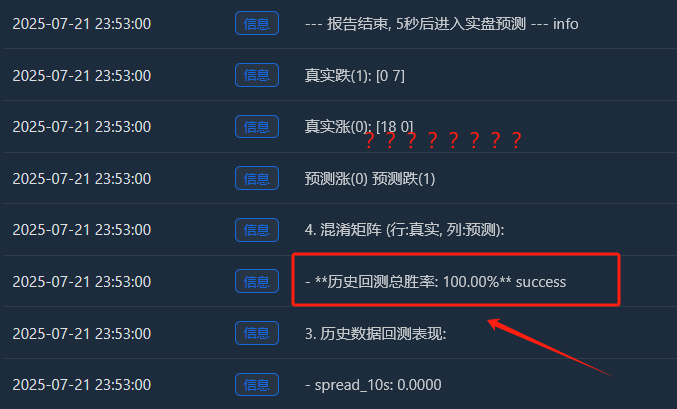
然后这个代码我运行 深度解读：为什么会出现“完美”的100%胜率？ 这个“完美”的结果，背后揭示了几个非常重要的、关于机器学习和金融市场的深刻道理。它不是一个Bug，而是一种在特定条件下会出现的、被称为“过拟合（Overfitting）”的典型现象。 “过拟合”是什么意思？

• 一个生动的比喻：想象一下，我们让一个学生（我们的SVM模型）去做一套非常短、而且题目类型非常单一的练习题（我们收集到的200根K线数据）。这个学生非常聪明，他没有去学习解题的通用方法，而是直接把这几道题的答案给死记硬背了下来。

• 结果：当我们用同一套练习题去考他时（这就是我们的“历史回测”），他当然能拿到100分的满分。但是，一旦我们给他一套全新的、他没见过的考题（未来的真实市场），他很可能一道都做不出来。

1. 为什么我们的模型会“过拟合”？

• 训练样本“太少”且“太特殊”:

• 虽然我们收集了200根K线（约3.3小时），但从日志看，最终筛选出的、符合我们定义的“有效涨跌”样本只有 18 + 7 = 25 个。

• 对于一个复杂的SVM模型来说，25个样本就如同汪洋大海中的几朵浪花，数量太少了。

• 更重要的是，这25个样本都来自于同一个下午的、一段高度相关的行情中。它们很可能拥有非常相似的“套路”。

1. 模型能力“太强”:

• SVM是一个非常强大的、非线性的分类器。它的能力就像一个拥有超强记忆力的大脑。
• 当强大的模型去学习一个过于简单和重复的数据集时，它就会倾向于“死记硬背”这些数据的所有细节和噪音，而不是去学习背后那个更具普适性的宏观规律。

1. 混淆矩阵的证据:

• 真实涨(0): [18 0] -> 18个上涨样本，全部完美记住。
• 真实跌(1): [0 7] -> 7个下跌样本，也全部完美记住。
• 这个完美的[ [18, 0], [0, 7] ]矩阵，就是模型“过拟合”的铁证。它几乎没有犯任何错误，这在充满随机性的金融市场中，本身就是一件“不正常”的事情。

所以，这个100%的胜率，我们应该这样解读：

“模型非常出色地学习并记忆了过去3个多小时这段特定行情下的所有规律。它证明了我们的特征工程和模型框架是有效的。但是，我们绝对不能指望它在未来的真实市场中，还能保持这么高的胜率。这更像是一次完美的‘随堂测验’，而不是‘高考’的最终成绩。”

机器学习也是我最近摸索的东西，我们下期在讲！ 对这个“偏科生”进行一次彻底的“思想改造”。我们的目标是：打破它的偏见，让它公正地、客观地看待“上涨”和“下跌”。