[TOC]

This article provides a practical, trading-oriented introduction to wavelet transform. The code examples are deliberately simplified for educational purposes, omitting more advanced procedures such as multi-level decomposition of standard wavelets, threshold-based denoising, and inverse transform reconstruction. Instead, it focuses on the core idea: using wavelet coefficients to perform multi-scale smoothing on price data in order to extract trend information. The approach is well suited for strategy development and rapid prototyping, but not intended for academic research or formal publication.

I. Introduction: Exposing the “Zhihu Gurus”

If you frequently browse quantitative finance topics on Zhihu, you’ve probably encountered scenes like this: Certain “gurus” love to throw around terms like:

• “Wavelet transform for denoising”
• “Fourier transform for extracting cycles”
• “Laplacian smoothing to remove outliers”

They make it sound so impressive that listeners are left completely dazzled, as if they’ve mastered the nuclear weapons of quantitative trading.

But ask them to show some code? “Well… it’s proprietary, can’t disclose that.”

Ask them to explain the underlying principles? “Well… it involves advanced mathematics, you wouldn’t understand anyway.”

Today, we’re going to explore exactly what these “Zhihu gurus” love to talk about. We’ll introduce the practical applications of wavelet transforms in financial markets, helping everyone develop a proper understanding of this technology.

II. What Exactly Is the Wavelet Transform?

An Intuitive Explanation

Imagine you are listening to a song, but the recording contains noise:

Original recording = vocals + background noise + electrical noise

The wavelet transform is like an intelligent filter:

• It keeps the vocals
• Filters out the noise
• And even tells you which time segment is the chorus and which is the verse

Now switch to financial markets:

Original price = true trend + short-term fluctuations + random noise

Wavelet transforms help you:

• Extract the true trend (long-term direction)
• Filter short-term fluctuations (intraday noise)
• Identify key turning points (trend reversals)

Core Concept: Basis Function Decomposition

At its core, the wavelet transform decomposes the original signal using a set of specific basis functions (wavelets).

Imagine describing a person’s appearance:

• Traditional method: describe each pixel one by one — extremely tedious
• Wavelet method: describe features like “eye size,” “nose height,” and “face contour,” then combine them

In financial prices:

Original price series = Basis function₁ × Weight₁ + Basis function₂ × Weight₂ + … + Noise

The basis functions are the “templates” corresponding to wavelet coefficients. Different wavelet types (Haar, Daubechies, Mexican Hat, etc.) use different templates — like using different “feature extractors” to decompose price movements.

Filters: Sieves in the Frequency Domain

A wavelet transform is essentially a multi-scale filter bank:

High-frequency filters → capture rapid fluctuations (intraday noise, tick-level jumps) Mid-frequency filters → capture medium-term trends (hours to days) Low-frequency filters → capture long-term trends (weekly or monthly direction)

Why Are They Called “Wavelets”?

• Traditional Fourier transforms use infinitely long sine waves — like an infinitely long ruler
• Wavelet transforms use finite-length “small” waves — like a set of rulers of different lengths

The problem with sine waves in financial markets: Sine waves assume periodic repetition, but financial markets are not periodic! BTC can rise 10% today and fall 8% tomorrow — no cycle at all.

The key advantage of wavelets is localization.

They can tell you:

“From 3:00 PM to 5:00 PM on December 20, 2025, price was mainly in an uptrend,”

instead of vague statements like “the market is ranging overall.”

Reconstruction: From Decomposition Back to the Original

Wavelet transforms are invertible, which is crucial.

Original price → wavelet decomposition → trend + fluctuation + noise Trend + fluctuation + noise → wavelet reconstruction → original price

Reconstruction means selectively recombining components:

After decomposition:

• Trend component = [99800, 99850, 99900, 99950, …] # what we want
• Fluctuation = [+200, -150, +180, -120, …] # potentially useful
• Noise = [±10, ±15, ±8, ±12, …] # discard!

During reconstruction, we only use the trend component:

• Reconstructed price = trend component + partial fluctuations

In real trading, we usually reconstruct only the low-frequency (trend) part and discard the high-frequency (noise) part. This is the essence of wavelet denoising.

Mathematical Principle (Simplified)

No heavy integrals — just plain language:

Wavelet transform = applying weighted averages to the price series using wavelet coefficients

Basic formula:

Smoothed price[i] = Σ(original price[i − j] × wavelet coefficient[j]) / Σ(wavelet coefficient[j])

From a filter perspective:

Original price → wavelet filter → components of different frequencies are “sifted out”

The key lies in choosing the wavelet coefficients:

• Different wavelets = different filter characteristics = different frequency responses
• Different levels = different time scales = different trend horizons

Example:

Suppose you use a Daubechies-4 wavelet with coefficients: [0.483, 0.837, 0.224, -0.129]

This set of coefficients defines a filter:

• Positive coefficients (0.483, 0.837, 0.224) → retain prices at those positions
• Negative coefficient (−0.129) → suppress earlier prices
• Coefficient weights → determine each price’s contribution

When you slide this filter across the entire price series, you perform the wavelet transform.

Each slide computes a weighted average over the current window — the weights are the wavelet coefficients.

Why Can It “Decompose” a Signal?

Because mathematically, any signal can be represented as a linear combination of wavelet basis functions.

Just like any color can be created by mixing RGB primary colors, any price series can be constructed from wavelet basis functions. Different wavelet types provide different “basis libraries,” suited to different kinds of signal analysis.

III. This Experiment: Practical Use of 7 Wavelet Transforms

Application Philosophy: Simplifying Theory for Practice

In signal-processing textbooks, wavelet analysis usually involves complex procedures:

Full wavelet analysis workflow:

• Multi-scale decomposition → approximation coefficients + detail coefficients
• Thresholding → soft/hard denoising of detail coefficients
• Inverse transform → reconstruct the signal
• Boundary extension → handle edge effects
• Energy normalization → ensure energy conservation

But in real financial trading, we don’t need all that complexity, because:

1. Trading Needs Direction, Not Perfect Reconstruction

Academic research may require reconstruction errors below 0.01%. In trading, we only need to know “up or down.”

Even with a 5% reconstruction error, as long as the trend direction is correct, the strategy can still be profitable.

1. Real-Time Constraints Require Simpler Computation

Full wavelet decomposition involves recursive multi-level calculations, which introduce latency in high-frequency trading. Direct convolution can be completed in milliseconds, meeting live trading requirements.

1. The Special Nature of Financial Signals

Financial prices are non-stationary and lack strict periodicity. Complex frequency decompositions add little value here — simple trend extraction is often more practical.

Simplified Strategy in This Study

This article extracts the essence of wavelet transforms and focuses only on what is most useful in financial markets:

• Core Simplification 1: Use Only Approximation Coefficients (Low-Frequency Trend)

Traditional wavelets: decompose → approximation + detail (multiple levels)

This approach: keep only approximation coefficients → directly obtain a smooth trend

• Core Simplification 2: Direct Convolution, No Threshold Denoising

Traditional wavelets: decompose → threshold detail coefficients → reconstruct

This approach: direct convolution → smoothed price

• Core Simplification 3: Ignore Boundary Handling

Traditional wavelets: require symmetric or periodic extension at boundaries

This approach: focus on the central region; boundary errors are acceptable

Implementation Method: Filter Convolution

def convolve(src, coeffs, step):
    """
    Core algorithm: apply wavelet coefficients to compute a weighted average
    over the price series
    
    src: price series [100000, 101000, 99000, ...]
    coeffs: wavelet coefficients [0.483, 0.837, 0.224, -0.129]
    step: sampling stride (used for multi-level scaling)
    """
    sum_val = 0.0   # weighted sum
    sum_w = 0.0     # sum of weights
    
    for i, weight in enumerate(coeffs):
        idx = i * step
        if idx < len(src):
            sum_val += src[idx] * weight
            sum_w += weight
    
    return sum_val / sum_w  # normalization

This function is the core of the wavelet filter:

• For each candlestick (K-line), it looks back N bars (where N = the number of wavelet coefficients)

• It uses the wavelet coefficients as weights to compute a weighted average

• By adjusting the step parameter, it achieves multi-level smoothing (Level 1 / Level 2 / Level 3 …)

Why Is This Simplification Reasonable?

Because the core objective of trading is simple:

Find the trend hidden inside noise.

The approximation coefficients of a wavelet transform are, by definition, a form of low-pass filtering. They preserve the low-frequency trend components of the signal — which is exactly what we need.

While a full wavelet analysis is mathematically more precise, in financial trading:

• Profits come from trend direction, not reconstruction accuracy

• Simpler methods are more robust; complex models are prone to overfitting

• Computation speed matters — in live trading, every millisecond costs money

Data Access: The Convenience of the FMZ Platform

Using the local backtesting engine of the FMZ (Inventors’ Quant) platform, data acquisition becomes extremely convenient.

'''backtest
start: 2025-12-17 00:00:00
end: 2025-12-23 08:00:00
period: 1h
basePeriod: 1h
exchanges: [{"eid":"Futures_Binance","currency":"BTC_USDT","fee":[0,0]}]
'''
from fmz import *

task = VCtx(__doc__)

def main():
    exchange.SetCurrency("BTC_USDT")
    exchange.SetContractType("swap")
    
    records = exchange.GetRecords(PERIOD_H1, 500)
    return records

records = main()

No complex API integration or data cleaning is required — we can directly obtain standardized candlestick (K-line) data. This allows us to quickly validate the real-world performance of seven wavelet types, instead of getting stuck in the swamp of data preprocessing.

Testing Objective

By comparing the performance of seven common wavelet types (Haar, Daubechies 4, Symlet 4, Biorthogonal 3.3, Mexican Hat, Morlet, Discrete Meyer) on cryptocurrency price data, we aim to visually demonstrate:

• The differences in smoothing strength across wavelets

• How the same wavelet behaves across different levels

• Which wavelets are better suited for short-term trading, and which are better for trend following

The focus is not on rigorous mathematical derivations, but on visual, practical results — helping traders build intuition and choose the wavelet type that best fits their own strategy.

IV. Detailed Breakdown of the 7 Wavelet Types

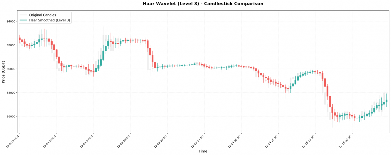
1. Haar Wavelet — The Simplest Average

The Haar wavelet is the most basic wavelet type. It has only two coefficients: [0.5, 0.5], which essentially means taking a simple average of two adjacent prices.

Core code:

coeffs = [0.5, 0.5]

# Apply to the price series [100000, 101000, 99000, 102000, 98000]
def smooth(prices, i):
    return (prices[i] * 0.5 + prices[i-1] * 0.5) / 1.0

# Result: [100000, 100500, 100000, 100500, 100000]

As you can see, the originally volatile price movement (from 99,000 to 102,000) becomes relatively smooth after applying the Haar wavelet.

This is the denoising effect of wavelets: they smooth out short-term, violent fluctuations, allowing you to see a cleaner and more stable price trajectory.

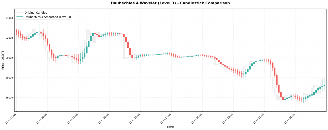
2. Daubechies 4 — The Engineering Workhorse

Daubechies 4 (abbreviated as db4) is one of the most commonly used wavelets in engineering applications. Its coefficients are:

Note that the last coefficient is negative, which is a distinctive characteristic of this wavelet.

Core code:

```python
coeffs = [0.483, 0.837, 0.224, -0.129]

# Process the i-th price point
def smooth(prices, i):
    weighted_sum = (prices[i]   * 0.483 +    # current price
                   prices[i-1] * 0.837 +     # 1 bar back, highest weight!
                   prices[i-2] * 0.224 +     # 2 bars back
                   prices[i-3] * (-0.129))   # 3 bars back, negative weight
    
    weight_sum = 0.483 + 0.837 + 0.224 + (-0.129)  # = 1.415
    return weighted_sum / weight_sum

# Example: smooth([100000, 101000, 99000, 102000], 3) ≈ 100251

Key characteristics: The weight of the previous candle (0.837) is even larger than that of the current price (0.483). This means db4 places more emphasis on what just happened in the market.

The negative coefficient applies a cancelling effect to older prices, which further enhances smoothness while preserving responsiveness.

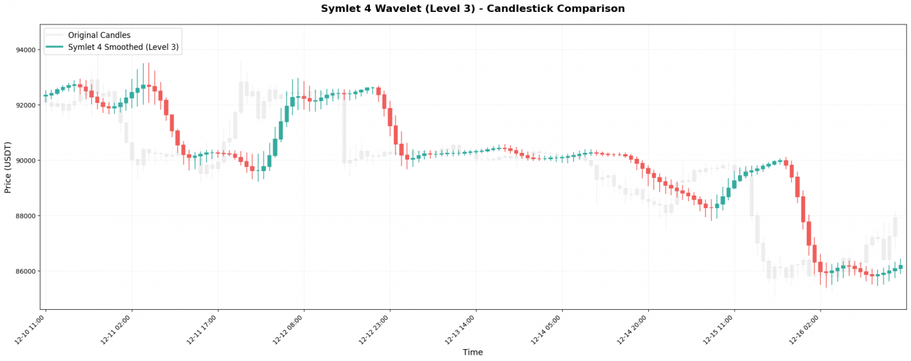
3. Symlet 4 - Symmetric Improved Version

Symlet 4 is an improved version of Daubechies, designed for better symmetry. Coefficients: [-0.076, -0.030, 0.498, 0.804, 0.298, -0.099, -0.013, 0.032].

Core code:

coeffs = [-0.076, -0.030, 0.498, 0.804, 0.298, -0.099, -0.013, 0.032]

# Look back over 8 candlesticks
def smooth(prices, i):
    weighted_sum = sum(prices[i-j] * coeffs[j] for j in range(8))
    weight_sum = sum(coeffs)
    return weighted_sum / weight_sum

# Produces stronger smoothing than Haar and db4,
# but with a slower response speed

Key characteristics: With a window length of 8 candlesticks, this wavelet has a much longer “memory” of past prices. As a result, a true trend reversal may only become visible on the smoothed curve after 8 candles, reflecting stronger smoothing but increased lag.

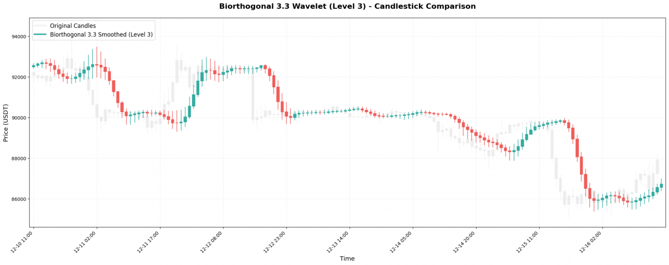
4. Biorthogonal 3.3 — Perfect Symmetry

Biorthogonal 3.3 (abbreviated as bior3.3) is a perfectly symmetric wavelet. Its coefficients are:

[-0.066, 0.283, 0.637, 0.283, -0.066]

Core code:

coeffs = [-0.066, 0.283, 0.637, 0.283, -0.066]
#           ↑              center ↑              ↑
#        perfectly symmetric ends

# Process the central price point
def smooth(prices, i):
    # Practical use: only look backward, no future data
    weighted_sum = (prices[i-4] * (-0.066) +   # 4 bars back
                   prices[i-3] * 0.283 +       # 3 bars back
                   prices[i-2] * 0.637 +       # 2 bars back, highest weight
                   prices[i-1] * 0.283 +       # 1 bar back
                   prices[i]   * (-0.066))     # current
    
    weight_sum = sum(coeffs)  # = 1.071
    return weighted_sum / weight_sum

Key characteristic: The symmetry guarantees no phase distortion — the smoothed curve will not inexplicably shift to the left or right in time.

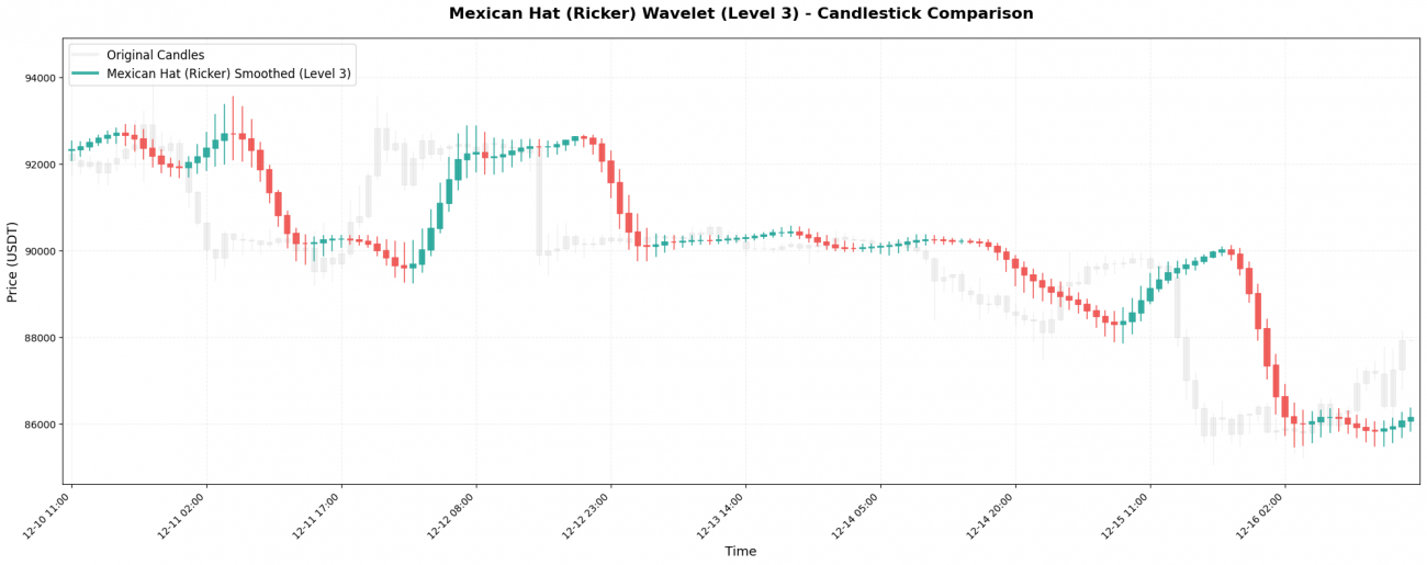
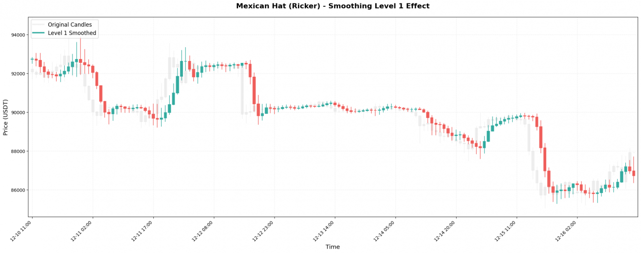
5. Mexican Hat — The Turning-Point Hunter

The Mexican Hat wavelet (also known as the Ricker wavelet) has coefficients:

[-0.1, 0.0, 0.4, 0.8, 0.4, 0.0, -0.1]

Its shape resembles a Mexican sombrero, hence the name.

Core code:

coeffs = [-0.1, 0.0, 0.4, 0.8, 0.4, 0.0, -0.1]
#         negative  zero  positive  max  positive  zero  negative
#         ↓                                    ↓
#   "penalizes" both ends, enhancing turning-point detection

def smooth(prices, i):
    weighted_sum = (prices[i-6] * (-0.1) +     # left 3, negative weight
                   prices[i-5] * 0.0 +         # left 2
                   prices[i-4] * 0.4 +         # left 1
                   prices[i-3] * 0.8 +         # center, highest weight
                   prices[i-2] * 0.4 +         # right 1
                   prices[i-1] * 0.0 +         # right 2
                   prices[i]   * (-0.1))       # right 3, negative weight
    
    weight_sum = sum(coeffs)
    return weighted_sum / weight_sum

Key characteristics: The “large center, negative ends” structure makes this wavelet particularly effective at detecting turning points — the critical moments when price shifts from rising to falling (or vice versa).

The negative coefficients penalize distant prices, allowing the wavelet to quickly capture changes in trend.

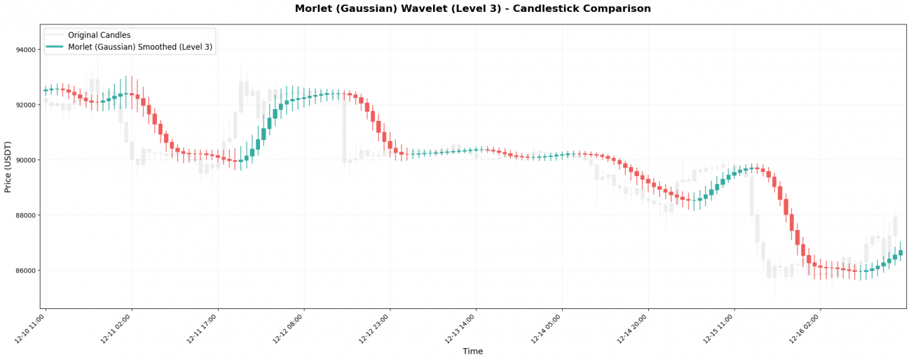
6. Morlet — The Gaussian Smoothing King

The Morlet wavelet is based on the Gaussian (normal) distribution. Its coefficients are:

[0.0625, 0.25, 0.375, 0.25, 0.0625]

Core code:

coeffs = [0.0625, 0.25, 0.375, 0.25, 0.0625]
#          ↓      ↓       ↓ center   ↓      ↓
#        far     near     highest    near     far
#        a perfect Gaussian bell curve

def smooth(prices, i):
    weighted_sum = (prices[i-4] * 0.0625 +     # left 2, 6.25%
                   prices[i-3] * 0.25 +        # left 1, 25%
                   prices[i-2] * 0.375 +       # center, 37.5%
                   prices[i-1] * 0.25 +        # right 1, 25%
                   prices[i]   * 0.0625)       # right 2, 6.25%
    
    # The weights sum exactly to 1.0, no division needed
    return weighted_sum

Key characteristics: The gentlest of all the wavelets — with no negative weights, every price point is smoothly and evenly incorporated into the calculation.

The resulting curve is extremely smooth, but the trade-off is slow responsiveness: sudden price changes may only appear after several candlesticks.

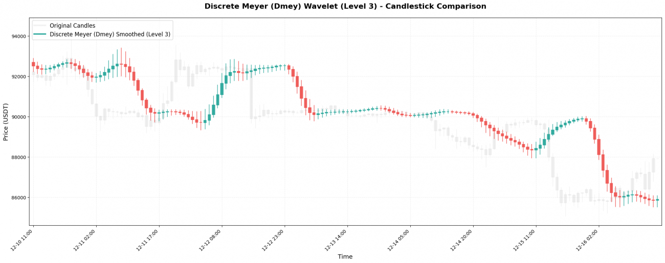
7. Discrete Meyer — Ultimate Smoothing

The Discrete Meyer wavelet is the most complex among these wavelets. Its coefficients are:

[-0.015, -0.025, 0.0, 0.28, 0.52, 0.28, 0.0, -0.025, -0.015]

Core code:

coeffs = [-0.015, -0.025, 0.0, 0.28, 0.52, 0.28, 0.0, -0.025, -0.015]
#           ↑       ↑            ↑    ↑ center ↑   ↑            ↑       ↑
#                     perfectly symmetric, center weight exceeds 50%

def smooth(prices, i):
    # Look back over 9 candlesticks
    weighted_sum = sum(prices[i-j] * coeffs[j] for j in range(9))
    weight_sum = sum(coeffs)  # = 1.0
    return weighted_sum

# Note: the weight on the 4-bars-back candle is 0.52, over 50%!
# This effectively tells you: "the mid-term trend from 4 bars ago"

Key characteristics: With the largest number of coefficients (9) and the longest historical lookback, this wavelet delivers the strongest smoothing.

It is well suited for extracting “weekly-level trends,” but at the cost of massive lag — by the time price has already fallen 10%, the smoothed curve may still be indicating “continued upside.”

V. Why Do Smoothing Effects Differ?

After reviewing the seven wavelets, a clear pattern emerges:

More coefficients = longer lookback = stronger smoothing = larger lag

Examples:

• Haar (2 coefficients) → looks back 1 bar → almost no smoothing

• Daubechies 4 (4 coefficients) → looks back 3 bars → light smoothing

• Mexican Hat (7 coefficients) → looks back 6 bars → medium smoothing

• Discrete Meyer (9 coefficients) → looks back 8 bars → heavy smoothing

The Role of Negative Weights

Negative coefficients = higher sensitivity = easier change detection

• Haar / Morlet (no negative weights) → gentle smoothing, low sensitivity

• Mexican Hat (negative weights at both ends) → highly sensitive to turning points

• Daubechies 4 (contains negative weight) → sensitive to trend changes

The Role of Symmetry

Symmetry = no distortion = shape preservation

• Asymmetric (Daubechies) → may shift left or right in time

• Symmetric (Biorthogonal / Meyer) → preserves the central position

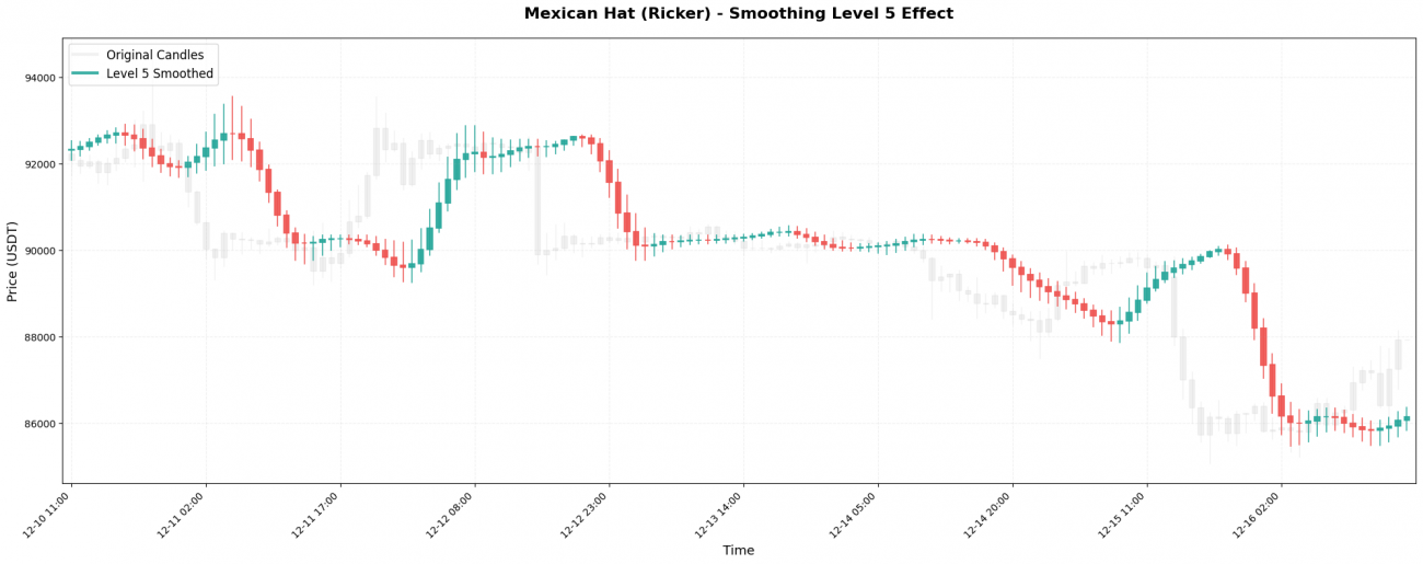
VI. The Impact of Smoothing Levels

Wavelet transforms can be applied recursively, like nested dolls. The first application is Level 1; applying the transform again to the Level-1 result produces Level 2, and so on.

Time Scales at Different Levels

Assume BTC trading on 1-hour candlesticks:

• Level 1 → captures 2–4 hour short-term fluctuations
• Level 2 → captures 4–8 hour trends
• Level 3 → captures 1–2 day medium-term trends (commonly used in strategies)
• Level 4 → captures 2–4 day swing moves
• Level 5 → captures 4–8 day major trends

Practical Comparison

Original BTC prices (1-hour bars): 99500, 99800, 99200, 100200, 99800, 100500, 100100, …

Level 1 result: 99600, 99650, 99500, 99900, 99950, 100200, 100250, … (slightly smoothed, fluctuations still visible)

Level 3 result: 99620, 99650, 99700, 99800, 99950, 100100, 100200, … (clearly smoother, shows the medium-term trend)

Level 5 result: 99630, 99640, 99660, 99700, 99760, 99840, 99930, … (extremely smooth, shows only the big-picture direction)

At higher levels, noise disappears almost entirely — but so does responsiveness. Choosing the right wavelet + the right level is ultimately a trade-off between clarity and timing, and should match the holding period and logic of your trading strategy.

Simple Selection Rule

The rule is straightforward:

Choose the Level that matches your holding period.

• 15-minute ultra-short-term trading → Level 1–2
• Intraday swing trading → Level 2–3
• Multi-day swing trades → Level 3–4
• Long-term trend following → Level 4–5

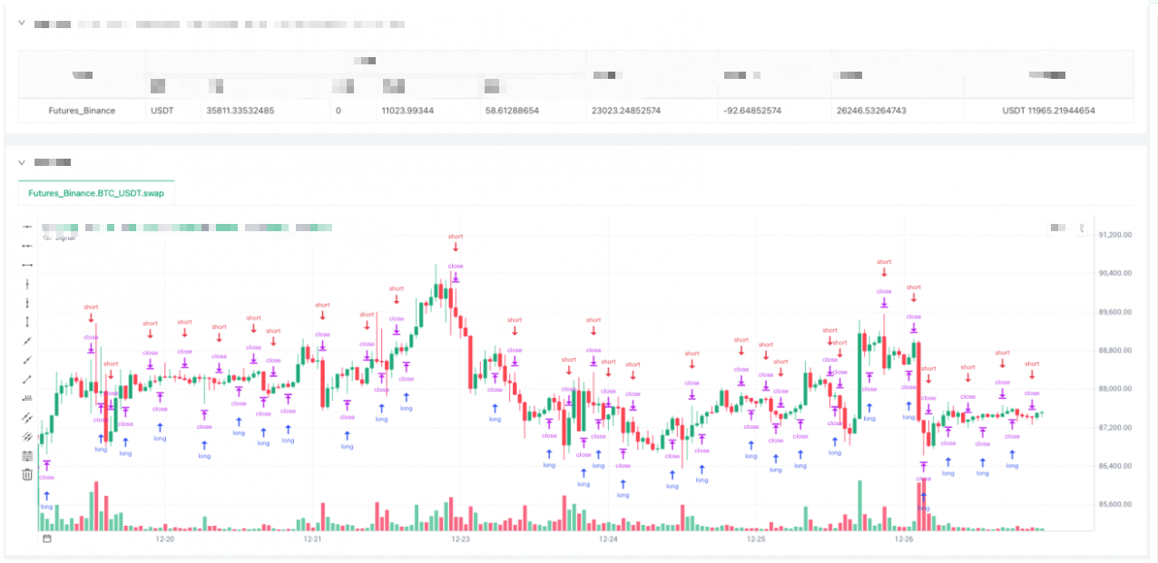
VII. Practical Application in Trading

The application of wavelet transforms in trading is very direct:

Use the smoothed price curve generated by the wavelet to determine trend direction, and trade when the trend changes.

Specifically:

If the smoothed close is higher than the previous one, the trend is up → go long

If the smoothed close is lower than the previous one, the trend is down → close longs or go short

This logic works because the wavelet transform has already filtered out short-term random fluctuations. What remains — “up” or “down” — is far more likely to represent a real trend change, rather than a false signal caused by noise.

# Execute wavelet transform
transformed = transformer.transform_ohlc(df)

# Get the smoothed closing prices of the last two candles
w_close_current = transformed['w_close'].values[-1]  # current smoothed close
w_close_prev = transformed['w_close'].values[-2]     # previous smoothed close

# Determine trend direction
signal = 0
if w_close_current > w_close_prev:
    signal = 1   # smoothed price rising → go long
elif w_close_current < w_close_prev:
    signal = -1  # smoothed price falling → go short

# Get account information
account = exchange.GetAccount()
ticker = exchange.GetTicker()

if not account or not ticker:
    Log("[Warning] Failed to get account/ticker info")
    Sleep(5000)
    continue

current_price = ticker['Last']

Log(f"[Price] Raw: {df['Close'].values[-1]:.2f}, "
    f"Smoothed (current): {w_close_current:.2f}, Smoothed (previous): {w_close_prev:.2f}")
Log(f"[Trend] {'↑ Uptrend' if signal == 1 else '↓ Downtrend' if signal == -1 else '→ Sideways'}")

# Execute trading logic
if signal == 1 and position != 1:
    # Smoothed price rising → go long
    Log(f"[Signal] Uptrend detected, opening long @ {current_price:.2f}")
    
    if position == -1:
        # Close short position first
        exchange.SetDirection("closesell")
        exchange.Buy(current_price, 1)
        Log(f"[Close] Closed short position")
    
    # Open long position
    exchange.SetDirection("buy")
    exchange.Buy(current_price, 1)
    Log(f"[Open] Opened long position")
    position = 1
    
elif signal == -1 and position != -1:
    # Smoothed price falling → go short
    Log(f"[Signal] Downtrend detected, opening short @ {current_price:.2f}")
    
    if position == 1:
        # Close long position first
        exchange.SetDirection("closebuy")
        exchange.Sell(current_price, 1)
        Log(f"[Close] Closed long position")
    
    # Open short position
    exchange.SetDirection("sell")
    exchange.Sell(current_price, 1)
    Log(f"[Open] Opened short position")
    position = -1

else:
    Log(f"[Position] Currently "
        f"{'Long' if position == 1 else 'Short' if position == -1 else 'Flat'}, no action needed")

Of course, real-world usage is never this simple or brute-force.

You can combine multiple wavelet levels at the same time. For example:

Level 2 to represent the short-term trend

Level 4 to represent the long-term trend

Only enter a position when both trends point in the same direction, which can significantly reduce false signals.

You can also introduce additional filters, such as:

Expanding trading volume

Sufficient volatility

Price breaking through a key level

All of these help improve the win rate.

For stop-loss management, you can dynamically set stops based on the volatility of the wavelet-smoothed price. For example:

Stop out if price falls below (smoothed price − 2 × ATR).

For position sizing, the clearer the trend (i.e., the steeper the slope of the smoothed price), the larger the position size. When the trend is unclear, reduce exposure or stay on the sidelines.

But the core idea never changes:

Use wavelets to turn noisy prices into clear trends, then make decisions on those trends.

This is far more reliable than reacting directly to raw candlesticks. Raw prices may rise 3% today, fall 2% tomorrow, then rise another 4% the day after — making it nearly impossible to tell whether the market is trending or ranging.

A wavelet-smoothed curve, however, tells you:

“Overall, price is moving upward during this period — despite intermediate fluctuations.”

VIII. Conclusion: A Rational View of the “Three Simple Tricks”

From a practical smoothing perspective, wavelet transforms do provide value in financial data processing:

They filter out part of the short-term noise

They help extract relatively clear trend information

However, they also have clear limitations:

Lag is unavoidable — wavelets operate purely on historical data

They cannot predict the future

Used alone, wavelet transforms are insufficient and must be combined with other analysis methods and risk controls to form a complete trading system

Why These Limitations Exist

The root cause lies in the unique nature of financial markets.

In traditional signal-processing domains such as speech recognition or image processing:

Noise characteristics are relatively stable

Signal patterns repeat consistently

Under these conditions, wavelet transforms excel at separating signal from noise.

Financial markets are fundamentally different:

What is considered “noise” today may become “signal” tomorrow

A model that works now may fail at any time in the future

Markets are non-stationary and dynamically evolving, with no permanent rules. This means that applying wavelet transforms in finance must always be adaptive and context-dependent.

A Simple Litmus Test for Overhyped Claims

When you encounter claims that excessively praise wavelet or Fourier transforms, try asking:

Which wavelet type was chosen?

Why that wavelet instead of others?

How was the smoothing level determined?

Are there corresponding backtest results and a documented parameter-selection process?

Anyone with genuine expertise should be able to clearly explain these technical choices.

Final Notes

Based on our limited but practical exploration, this study aims to present wavelet transforms in an accessible way, helping readers build a basic, intuitive understanding of how they can be applied in trading.

We maintain deep respect for quantitative researchers who work extensively in this field. If you are an expert, we warmly welcome corrections and suggestions — such as:

Theoretical foundations for wavelet parameter selection

Optimization of multi-scale combinations

Implementation paths for adaptive wavelet selection

We will gladly incorporate constructive feedback and continue refining this work.

Plotting function: implemented using the FMZ local backtesting engine

'''backtest
start: 2025-12-17 00:00:00
end: 2025-12-23 08:00:00
period: 1h
basePeriod: 1h
exchanges: [{"eid":"Futures_Binance","currency":"BTC_USDT","fee":[0,0]}]
'''
from fmz import *
import numpy as np
import pandas as pd
import matplotlib.pyplot as plt
from matplotlib.patches import Rectangle

task = VCtx(__doc__)

# ==================== Wavelet Coefficient Library ====================
class WaveletCoefficients:
    """Wavelet Coefficients Definition"""
    
    @staticmethod
    def get_coeffs(wavelet_name):
        """Get coefficients for different wavelet types"""
        coeffs = {
            "Haar": [0.5, 0.5],
            
            "Daubechies 4": [
                0.48296291314453414,
                0.8365163037378079,
                0.22414386804201339,
                -0.12940952255126037
            ],
            
            "Symlet 4": [
                -0.05357, -0.02096, 0.35238,
                0.56833, 0.21062, -0.07007,
                -0.01941, 0.03268
            ],
            
            "Biorthogonal 3.3": [
                -0.06629, 0.28289, 0.63678,
                0.28289, -0.06629
            ],
            
            "Mexican Hat (Ricker)": [
                -0.1, 0.0, 0.4, 0.8, 0.4, 0.0, -0.1
            ],
            
            "Morlet (Gaussian)": [
                0.0625, 0.25, 0.375, 0.25, 0.0625
            ],
            
            "Discrete Meyer (Dmey)": [
                -0.015, -0.025, 0.0,
                0.28, 0.52, 0.28,
                0.0, -0.025, -0.015
            ]
        }
        
        return coeffs.get(wavelet_name, coeffs["Mexican Hat (Ricker)"])


# ==================== Wavelet Transform Engine ====================
class WaveletTransform:
    """Wavelet Transform Engine"""
    
    def __init__(self, wavelet_type="Mexican Hat (Ricker)", smoothing_level=3):
        self.wavelet_type = wavelet_type
        self.smoothing_level = smoothing_level
        self.coeffs = WaveletCoefficients.get_coeffs(wavelet_type)
    
    def convolve(self, src, coeffs, step):
        """
        Convolution operation - Core algorithm
        
        Args:
            src: Source data sequence
            coeffs: Wavelet coefficients
            step: Sampling step
        
        Returns:
            Convolved value
        """
        sum_val = 0.0
        sum_w = 0.0
        
        for i, weight in enumerate(coeffs):
            idx = i * step
            if idx < len(src):
                val = src[idx]
                sum_val += val * weight
                sum_w += weight
        
        # Normalization - critical fix
        return sum_val / sum_w if sum_w != 0 else sum_val
    
    def calc_level(self, data, target_level):
        """
        Calculate wavelet transform for the specified level
        
        Args:
            data: Original data array
            target_level: Target smoothing level
        
        Returns:
            Transformed data array
        """
        result = []
        coeffs = self.coeffs
        
        for i in range(len(data)):
            # Retrieve historical data backwards from the current index
            src = data[max(0, i - 50):i + 1][::-1]
            
            # Level 1
            val = self.convolve(src, coeffs, 1)
            
            # Level 2
            if target_level >= 2:
                src_temp = [val] + [
                    self.convolve(
                        data[max(0, j - 50):j + 1][::-1], coeffs, 1
                    ) for j in range(max(0, i - 10), i)
                ][::-1]
                val = self.convolve(src_temp, coeffs, 2)
            
            # Level 3
            if target_level >= 3:
                val = self.convolve([val] * len(coeffs), coeffs, 4)
            
            # Level 4+
            if target_level >= 4:
                val = self.convolve([val] * len(coeffs), coeffs, 8)
            
            result.append(val)
        
        return np.array(result)
    
    def transform_ohlc(self, df):
        """
        Perform wavelet transform on OHLC data
        
        Args:
            df: DataFrame with Open / High / Low / Close
        
        Returns:
            Transformed DataFrame
        """
        result_df = df.copy()
        
        # Transform each price series
        result_df['w_open'] = self.calc_level(df['Open'].values, self.smoothing_level)
        result_df['w_high'] = self.calc_level(df['High'].values, self.smoothing_level)
        result_df['w_low'] = self.calc_level(df['Low'].values, self.smoothing_level)
        result_df['w_close'] = self.calc_level(df['Close'].values, self.smoothing_level)
        
        # Reconstruct logically consistent candlesticks
        result_df['real_high'] = result_df[
            ['w_high', 'w_low', 'w_open', 'w_close']
        ].max(axis=1)
        result_df['real_low'] = result_df[
            ['w_high', 'w_low', 'w_open', 'w_close']
        ].min(axis=1)
        
        return result_df


# ==================== Candlestick Visualization Tool ====================
class WaveletCandlestickVisualizer:
    """Wavelet Candlestick Visualization"""
    
    @staticmethod
    def plot_single_wavelet(df, wavelet_type, smoothing_level=3, n_bars=200):
        """
        Plot comparison for a single wavelet type
        
        Args:
            df: Original candlestick data
            wavelet_type: Wavelet type
            smoothing_level: Smoothing level
            n_bars: Number of bars to display
        """
        # Use only the last n_bars
        df_plot = df.iloc[-n_bars:].copy()
        
        # Create figure
        fig, ax = plt.subplots(figsize=(20, 8))
        
        # Perform wavelet transform
        transformer = WaveletTransform(wavelet_type, smoothing_level)
        transformed = transformer.transform_ohlc(df)
        transformed_plot = transformed.iloc[-n_bars:].copy()
        
        # Draw original candlesticks (gray background)
        WaveletCandlestickVisualizer._draw_candlesticks(
            ax, df_plot, 
            color_up='lightgray', 
            color_down='lightgray',
            alpha=0.3,
            label='Original Candles'
        )
        
        # Draw wavelet-smoothed candlesticks
        WaveletCandlestickVisualizer._draw_candlesticks(
            ax, transformed_plot,
            use_wavelet=True,
            color_up='#26A69A',  # Green
            color_down='#EF5350',  # Red
            alpha=0.9,
            linewidth=1.2,
            label=f'{wavelet_type} Smoothed (Level {smoothing_level})'
        )
        
        # Set title and labels
        ax.set_title(
            f'{wavelet_type} Wavelet (Level {smoothing_level}) - Candlestick Comparison',
            fontsize=16, fontweight='bold', pad=20
        )
        ax.set_ylabel('Price (USDT)', fontsize=13)
        ax.set_xlabel('Time', fontsize=13)
        ax.grid(True, alpha=0.2, linestyle='--')
        ax.legend(loc='upper left', fontsize=12)
        
        # Format x-axis
        ax.set_xlim(-1, len(df_plot))
        ax.set_xticks(range(0, len(df_plot), max(1, len(df_plot) // 10)))
        ax.set_xticklabels(
            [df_plot.index[i].strftime('%m-%d %H:%M')
             for i in range(0, len(df_plot), max(1, len(df_plot) // 10))],
            rotation=45, ha='right'
        )
        
        plt.tight_layout()
        plt.show()
        return fig
    
    @staticmethod
    def plot_single_level(df, wavelet_type, level, n_bars=200):
        """
        Plot comparison for a single smoothing level
        
        Args:
            df: Original candlestick data
            wavelet_type: Wavelet type
            level: Smoothing level
            n_bars: Number of bars to display
        """
        # Use only the last n_bars
        df_plot = df.iloc[-n_bars:].copy()
        
        # Create figure
        fig, ax = plt.subplots(figsize=(20, 8))
        
        # Perform wavelet transform
        transformer = WaveletTransform(wavelet_type, level)
        transformed = transformer.transform_ohlc(df)
        transformed_plot = transformed.iloc[-n_bars:].copy()
        
        # Draw original candlesticks
        WaveletCandlestickVisualizer._draw_candlesticks(
            ax, df_plot,
            color_up='lightgray',
            color_down='lightgray',
            alpha=0.3,
            label='Original Candles'
        )
        
        # Draw wavelet-smoothed candlesticks
        WaveletCandlestickVisualizer._draw_candlesticks(
            ax, transformed_plot,
            use_wavelet=True,
            color_up='#26A69A',
            color_down='#EF5350',
            alpha=0.9,
            linewidth=1.2,
            label=f'Level {level} Smoothed'
        )
        
        # Set title and labels
        ax.set_title(
            f'{wavelet_type} - Smoothing Level {level} Effect',
            fontsize=16, fontweight='bold', pad=20
        )
        ax.set_ylabel('Price (USDT)', fontsize=13)
        ax.set_xlabel('Time', fontsize=13)
        ax.grid(True, alpha=0.2, linestyle='--')
        ax.legend(loc='upper left', fontsize=12)
        
        # Format x-axis
        ax.set_xlim(-1, len(df_plot))
        ax.set_xticks(range(0, len(df_plot), max(1, len(df_plot) // 10)))
        ax.set_xticklabels(
            [df_plot.index[i].strftime('%m-%d %H:%M')
             for i in range(0, len(df_plot), max(1, len(df_plot) // 10))],
            rotation=45, ha='right'
        )
        
        plt.tight_layout()
        plt.show()
        return fig
    
    @staticmethod
    def _draw_candlesticks(ax, df, use_wavelet=False, color_up='green', 
                           color_down='red', alpha=1.0, linewidth=1.0, label=''):
        """
        Draw candlestick chart
        
        Args:
            ax: Matplotlib axis
            df: Data DataFrame
            use_wavelet: Whether to use wavelet-transformed data
            color_up: Up candle color
            color_down: Down candle color
            alpha: Transparency
            linewidth: Line width
            label: Legend label
        """
        if use_wavelet:
            opens = df['w_open'].values
            highs = df['real_high'].values
            lows = df['real_low'].values
            closes = df['w_close'].values
        else:
            opens = df['Open'].values
            highs = df['High'].values
            lows = df['Low'].values
            closes = df['Close'].values
        
        for i in range(len(df)):
            x = i
            open_price = opens[i]
            high_price = highs[i]
            low_price = lows[i]
            close_price = closes[i]
            
            color = color_up if close_price >= open_price else color_down
            
            # Draw wick
            ax.plot(
                [x, x],
                [low_price, high_price],
                color=color,
                linewidth=linewidth,
                alpha=alpha
            )
            
            # Draw body
            height = abs(close_price - open_price)
            bottom = min(open_price, close_price)
            
            rect = Rectangle(
                (x - 0.3, bottom),
                0.6,
                height,
                facecolor=color,
                edgecolor=color,
                alpha=alpha,
                linewidth=linewidth
            )
            ax.add_patch(rect)
        
        # Add legend placeholder (only once)
        if label:
            ax.plot([], [], color=color_up, linewidth=3, alpha=alpha, label=label)


# ==================== Main Function ====================
def main():
    """Main execution flow"""
    exchange.SetCurrency("BTC_USDT")
    exchange.SetContractType("swap")
    
    # Retrieve candlestick data
    records = exchange.GetRecords(PERIOD_H1, 500)
    
    # Convert to DataFrame
    df = pd.DataFrame(
        records,
        columns=['Time', 'Open', 'High', 'Low', 'Close', 'Volume']
    )
    df['Time'] = pd.to_datetime(df['Time'], unit='ms')
    df.set_index('Time', inplace=True)
    
    print(f"Data loaded: {len(df)} bars")
    print(f"Time range: {df.index[0]} to {df.index[-1]}")
    print(f"Price range: ${df['Low'].min():.2f} - ${df['High'].max():.2f}")
    
    return df


# ==================== Execute Plotting ====================
try:
    # Load candlestick data
    kline = main()
    
    print("\n" + "=" * 70)
    print("Generating Wavelet Candlestick Charts (Each in Separate Window)...")
    print("=" * 70)
    
    # ========== Chart Series 1: Different Wavelet Types ==========
    print("\n[Series 1] Comparing Different Wavelet Types")
    print("-" * 70)
    
    wavelet_types = [
        "Haar",
        "Daubechies 4",
        "Symlet 4",
        "Biorthogonal 3.3",
        "Mexican Hat (Ricker)",
        "Morlet (Gaussian)",
        "Discrete Meyer (Dmey)"  # Discrete Meyer added
    ]
    
    for i, wavelet_type in enumerate(wavelet_types, 1):
        print(f"  Chart {i}/{len(wavelet_types)}: {wavelet_type}")
        fig = WaveletCandlestickVisualizer.plot_single_wavelet(
            kline,
            wavelet_type=wavelet_type,
            smoothing_level=3,
            n_bars=150
        )
    
    # ========== Chart Series 2: Different Smoothing Levels ==========
    print("\n[Series 2] Comparing Different Smoothing Levels")
    print("-" * 70)
    
    levels = [1, 2, 3, 4, 5]
    
    for i, level in enumerate(levels, 1):
        print(f"  Chart {i}/5: Level {level}")
        fig = WaveletCandlestickVisualizer.plot_single_level(
            kline,
            wavelet_type="Mexican Hat (Ricker)",
            level=level,
            n_bars=150
        )
    
    print("\n" + "=" * 70)
    print("All charts generated successfully!")
    print(
        f"Total charts: {len(wavelet_types) + len(levels)} "
        f"({len(wavelet_types)} wavelets + {len(levels)} levels)"
    )
    print("=" * 70)
    
except Exception as e:
    print(f"Error: {str(e)}")
    import traceback
    print(traceback.format_exc())
finally:
    print("\nStrategy testing completed.")

Trading functions: applied on the FMZ platform

'''backtest
start: 2025-01-17 00:00:00
end: 2025-12-23 08:00:00
period: 1h
basePeriod: 1h
exchanges: [{"eid":"Futures_Binance","currency":"BTC_USDT","fee":[0,0]}]
'''

import numpy as np
import pandas as pd

# ==================== Wavelet Coefficient Library ====================
class WaveletCoefficients:
    """Same as the previous section"""

# ==================== Wavelet Transform Engine ====================
class WaveletTransform:
    """Same as the previous section"""
 
def main():
    """Wavelet Trading Main Function - Based on Smoothed Price Trend"""
    
    # ========== Configuration Parameters ==========
    WAVELET_TYPE = "Mexican Hat (Ricker)"  # Wavelet type
    SMOOTHING_LEVEL = 1                     # Smoothing level
    
    # Initialization
    exchange.SetCurrency("BTC_USDT")
    exchange.SetContractType("swap")
    
    Log(f"=" * 70)
    Log(f"Wavelet Trend Following Strategy")
    Log(f"Wavelet: {WAVELET_TYPE}, Level: {SMOOTHING_LEVEL}")
    Log(f"Logic: Smoothed close up → go long, Smoothed close down → go short")
    Log(f"=" * 70)
    
    # Initialize wavelet transformer
    transformer = WaveletTransform(WAVELET_TYPE, SMOOTHING_LEVEL)
    
    # Position state
    position = 0  # 0: no position, 1: long, -1: short
    
    while True:

        # Get candlestick data
        records = exchange.GetRecords(PERIOD_H1, 500)
        if not records:
            Log("[Warning] Failed to get kline data")
            Sleep(5000)
            continue
        
        df = pd.DataFrame(records, columns=['Time', 'Open', 'High', 'Low', 'Close', 'Volume'])
        df['Time'] = pd.to_datetime(df['Time'], unit='ms')
        df.set_index('Time', inplace=True)
        
        # Perform wavelet transform
        transformed = transformer.transform_ohlc(df)
        
        # Get the last two smoothed closing prices
        w_close_current = transformed['w_close'].values[-1]  # Current smoothed close
        w_close_prev = transformed['w_close'].values[-2]     # Previous smoothed close
        
        # Determine trend direction
        signal = 0
        if w_close_current > w_close_prev:
            signal = 1   # Smoothed price rising → go long
        elif w_close_current < w_close_prev:
            signal = -1  # Smoothed price falling → go short
        
        # Get account and market info
        account = exchange.GetAccount()
        ticker = exchange.GetTicker()
        
        if not account or not ticker:
            Log("[Warning] Failed to get account/ticker info")
            Sleep(5000)
            continue
        
        current_price = ticker['Last']
        
        Log(f"[Price] Raw: {df['Close'].values[-1]:.2f}, "
            f"Smoothed current: {w_close_current:.2f}, Smoothed previous: {w_close_prev:.2f}")
        Log(f"[Trend] {'↑ Uptrend' if signal == 1 else '↓ Downtrend' if signal == -1 else '→ Sideways'}")
        
        # Trading logic
        if signal == 1 and position != 1:
            # Smoothed price rising → go long
            Log(f"[Signal] Uptrend detected, open long @ {current_price:.2f}")
            
            if position == -1:
                # Close short position first
                exchange.SetDirection("closesell")
                exchange.Buy(current_price, 1)
                Log(f"[Close] Short position closed")
            
            # Open long position
            exchange.SetDirection("buy")
            exchange.Buy(current_price, 1)
            Log(f"[Open] Long position opened")
            position = 1
            
        elif signal == -1 and position != -1:
            # Smoothed price falling → go short
            Log(f"[Signal] Downtrend detected, open short @ {current_price:.2f}")
            
            if position == 1:
                # Close long position first
                exchange.SetDirection("closebuy")
                exchange.Sell(current_price, 1)
                Log(f"[Close] Long position closed")
            
            # Open short position
            exchange.SetDirection("sell")
            exchange.Sell(current_price, 1)
            Log(f"[Open] Short position opened")
            position = -1
        
        else:
            Log(f"[Position] Current state: "
                f"{'Long' if position == 1 else 'Short' if position == -1 else 'Flat'}, no action required")
        
        Log(f"[Account] Balance: {account['Balance']:.2f}, Equity: {account['Equity']:.2f}")
        Log("-" * 70)
        
        Sleep(60000 * 60)