多层次斐波那契趋势跟踪与对冲交易策略系统

[tran]

概述

多层次斐波那契趋势跟踪与对冲交易策略系统是一个集成了多种技术分析指标的综合性量化交易策略。该策略以斐波那契回撤理论为核心，结合指数移动平均线(EMA)、平均真实波幅(ATR)、平均趋向指数(ADX)以及方向性移动指标(DMI)等多个技术指标，构建了一个多维度的市场分析框架。策略不仅具备传统的趋势跟踪功能，还集成了反弹交易机制和对冲功能，旨在不同市场条件下都能够捕获盈利机会并有效控制风险。

该策略的独特之处在于其多层次的风险管理体系和灵活的交易模式。通过设置多个止盈目标(TP1和TP2)和基于ATR的动态止损机制，策略能够在保护资本的同时最大化收益潜力。此外，内置的对冲功能为策略增加了额外的风险缓冲，使其在波动性较大的市场环境中也能保持相对稳定的表现。

策略原理

策略的核心逻辑基于斐波那契回撤理论与趋势分析的结合。首先，策略通过计算指定周期内的最高点和最低点来确定斐波那契回撤水平，包括23.6%、38.2%、50%、61.8%、78.6%、100%和161.8%等关键位置。这些水平被用作重要的支撑和阻力位，为交易信号的生成提供关键参考。

在趋势识别方面，策略采用50期指数移动平均线作为主要的趋势判断工具。当价格连续三根K线都位于EMA上方时，被认定为上升趋势；反之则为下降趋势。同时，策略还分析价格结构，通过识别更高的低点和更高的高点来确认多头结构，通过更低的高点和更低的低点来确认空头结构。

ADX和DMI指标的引入增强了趋势强度的判断精确度。ADX值大于20被视为强趋势的标准，而+DI和-DI的相对强弱则用于确定趋势的方向性。成交量分析也是策略的重要组成部分，当成交量超过20期平均值的1.2倍时，被认为是有效的量能确认。

交易信号的生成需要满足多个条件的同时成立：趋势方向明确、价格接近关键斐波那契水平、趋势强度充足、方向性指标确认以及成交量放大。这种多重过滤机制大大提高了信号的可靠性，降低了假信号的概率。

策略优势

该策略具有多项显著优势，首先体现在其综合性的技术分析框架。通过整合斐波那契理论、趋势分析、动量指标和成交量分析，策略能够从多个维度评估市场状况，提供更加全面和准确的交易信号。这种多指标融合的方法有效减少了单一指标可能产生的误导性信号，提高了整体策略的稳定性和可靠性。

策略的风险管理体系是其另一大优势。双重止盈机制允许交易者在达到第一个目标时锁定部分利润，同时保留剩余仓位追求更大收益。基于ATR的动态止损设置能够根据市场波动性自动调整风险控制水平，既能在低波动时收紧止损以保护利润，又能在高波动时放宽止损以避免被正常波动震出。

反弹交易功能为策略增加了额外的盈利机会。当价格在关键支撑或阻力位发生反弹时，策略能够快速识别并参与这种短期逆转行情，从而在趋势交易的基础上增加更多的交易机会。这种灵活性使策略能够适应不同的市场条件，无论是强趋势市场还是区间震荡市场都能找到合适的交易机会。

对冲功能的集成是该策略的一个创新特色。当持有多头仓位时若出现空头信号，策略会开启对冲空头仓位；反之亦然。这种机制能够在市场快速反转时提供额外保护，减少潜在损失并可能转化为新的盈利机会。

时间过滤器的设置防止了过度交易的问题。通过要求连续信号之间至少间隔5根K线，策略避免了在短时间内频繁开仓，降低了交易成本并提高了信号质量。

策略风险

尽管该策略具有多项优势，但仍存在一些需要注意的风险因素。首先是参数依赖性风险。策略涉及多个参数设置，包括斐波那契周期、容忍度、ATR倍数等，这些参数的选择对策略表现有重要影响。不当的参数设置可能导致过度拟合历史数据或在实际市场中表现不佳。因此，需要通过充分的回测和参数优化来找到最适合特定市场和时间框架的参数组合。

市场环境适应性是另一个潜在风险。策略主要基于技术分析，在某些市场条件下可能表现不佳，例如在基本面驱动的强烈单边行情中，技术指标可能会失效。此外，在极低波动性或极高波动性的市场环境中，策略的信号生成频率和准确性都可能受到影响。

滑点和执行风险也需要考虑。在实际交易中，特别是在波动性较大的市场条件下，可能存在订单执行价格与期望价格之间的差异。这种滑点成本可能会侵蚀策略的理论收益，特别是对于频繁交易的策略。

对冲功能虽然提供了额外保护，但也增加了策略的复杂性。在某些情况下，对冲操作可能会导致多空仓位同时亏损，或者在手续费方面产生额外成本。因此，需要谨慎评估对冲功能的实际效果，并考虑在特定市场条件下是否启用该功能。

策略优化方向

为了进一步提升策略性能，可以从多个方向进行优化。首先是动态参数调整机制的引入。可以根据市场波动性、趋势强度等因素动态调整斐波那契周期、ATR倍数等关键参数。例如，在高波动市场中增加ATR倍数以提供更大的止损空间，在低波动市场中减少ATR倍数以收紧风险控制。

机器学习技术的整合是另一个重要的优化方向。可以使用机器学习算法来识别最佳的入场时机，或者根据历史数据学习参数组合的最优配置。此外，还可以利用自然语言处理技术分析市场情绪和新闻事件对价格的影响，为策略增加基本面分析维度。

多时间框架分析的集成能够提供更全面的市场视角。可以在更长的时间框架上确认大趋势方向，在较短的时间框架上寻找精确的入场点。这种多时间框架的协调分析能够提高信号质量并减少逆势交易的风险。

资金管理优化也是提升策略表现的重要途径。可以根据市场条件、策略信心度等因素动态调整仓位大小。例如，在高信心度信号时增加仓位，在低信心度信号时减少仓位。此外，还可以引入最大回撤控制机制，当策略出现较大亏损时自动减少仓位或暂停交易。

止盈止损逻辑的进一步精细化也值得考虑。可以引入追踪止损机制，根据价格走势动态调整止损位置以锁定更多利润。同时，可以根据市场结构特征设置更加智能的止盈目标，例如在关键阻力位附近提前止盈。

总结

多层次斐波那契趋势跟踪与对冲交易策略系统代表了现代量化交易技术的一个重要发展方向。该策略通过巧妙地整合多种经典技术分析工具，构建了一个既稳健又灵活的交易框架。其多重过滤机制确保了信号质量，多层次风险管理体系提供了有效的资本保护，而对冲功能则为策略增加了额外的安全边际。

策略的成功实施需要充分理解其基本原理和运作机制，并根据具体的交易环境进行适当的参数调整和优化。虽然该策略在理论上具有良好的设计，但实际应用中仍需要考虑市场微观结构、交易成本、滑点等现实因素的影响。

随着人工智能和机器学习技术的不断发展，该策略还有巨大的优化空间。通过引入更先进的数据分析技术和自适应机制，策略的性能有望得到进一步提升。对于量化交易者而言，这类综合性策略提供了一个宝贵的学习和改进平台，有助于深入理解市场动态和风险管理的重要性。 ||

Overview

The Multi-Level Fibonacci Trend Following and Hedging Trading Strategy System is a comprehensive quantitative trading strategy that integrates multiple technical analysis indicators. This strategy centers on Fibonacci retracement theory, combining Exponential Moving Average (EMA), Average True Range (ATR), Average Directional Index (ADX), and Directional Movement Indicator (DMI) to construct a multi-dimensional market analysis framework. The strategy not only features traditional trend-following capabilities but also integrates bounce trading mechanisms and hedging functionality, aiming to capture profitable opportunities under different market conditions while effectively controlling risk.

The unique aspect of this strategy lies in its multi-layered risk management system and flexible trading modes. By setting multiple take-profit targets (TP1 and TP2) and dynamic stop-loss mechanisms based on ATR, the strategy can maximize profit potential while protecting capital. Additionally, the built-in hedging function adds an extra risk buffer to the strategy, enabling it to maintain relatively stable performance even in highly volatile market environments.

Strategy Principles

The core logic of the strategy is based on the combination of Fibonacci retracement theory and trend analysis. First, the strategy calculates the highest and lowest points within a specified period to determine Fibonacci retracement levels, including key positions at 23.6%, 38.2%, 50%, 61.8%, 78.6%, 100%, and 161.8%. These levels serve as important support and resistance zones, providing crucial references for trading signal generation.

For trend identification, the strategy employs a 50-period Exponential Moving Average as the primary trend determination tool. When prices remain above the EMA for three consecutive candlesticks, it’s identified as an uptrend; conversely, it’s considered a downtrend. Simultaneously, the strategy analyzes price structure by identifying higher lows and higher highs to confirm bullish structure, and lower highs and lower lows to confirm bearish structure.

The introduction of ADX and DMI indicators enhances the precision of trend strength assessment. An ADX value greater than 20 is considered the standard for a strong trend, while the relative strength of +DI and -DI is used to determine trend direction. Volume analysis is also an important component of the strategy, where volume exceeding 1.2 times the 20-period average is considered effective volume confirmation.

Trade signal generation requires multiple conditions to be met simultaneously: clear trend direction, price proximity to key Fibonacci levels, sufficient trend strength, directional indicator confirmation, and volume expansion. This multi-filter mechanism significantly improves signal reliability and reduces the probability of false signals.

Strategy Advantages

This strategy possesses multiple significant advantages, first manifested in its comprehensive technical analysis framework. By integrating Fibonacci theory, trend analysis, momentum indicators, and volume analysis, the strategy can evaluate market conditions from multiple dimensions, providing more comprehensive and accurate trading signals. This multi-indicator fusion approach effectively reduces misleading signals that might be generated by single indicators, improving the overall stability and reliability of the strategy.

The strategy’s risk management system represents another major advantage. The dual take-profit mechanism allows traders to lock in partial profits upon reaching the first target while maintaining remaining positions to pursue greater returns. ATR-based dynamic stop-loss settings can automatically adjust risk control levels according to market volatility, tightening stops during low volatility to protect profits and relaxing stops during high volatility to avoid being stopped out by normal fluctuations.

The bounce trading functionality adds additional profit opportunities to the strategy. When prices bounce at key support or resistance levels, the strategy can quickly identify and participate in such short-term reversal movements, thereby adding more trading opportunities beyond trend trading. This flexibility enables the strategy to adapt to different market conditions, finding suitable trading opportunities whether in strong trending markets or range-bound markets.

The integration of hedging functionality is an innovative feature of this strategy. When holding long positions and a short signal appears, the strategy will open a hedge short position; vice versa. This mechanism can provide additional protection during rapid market reversals, reducing potential losses and possibly converting them into new profit opportunities.

The time filter setting prevents overtrading issues. By requiring at least 5 candlesticks between consecutive signals, the strategy avoids frequent position opening within short periods, reducing trading costs and improving signal quality.

Strategy Risks

Despite the strategy’s multiple advantages, several risk factors require attention. First is parameter dependency risk. The strategy involves multiple parameter settings, including Fibonacci period, tolerance, ATR multipliers, etc. The selection of these parameters significantly impacts strategy performance. Inappropriate parameter settings may lead to overfitting historical data or poor performance in actual markets. Therefore, sufficient backtesting and parameter optimization are needed to find the most suitable parameter combinations for specific markets and timeframes.

Market environment adaptability represents another potential risk. The strategy is primarily based on technical analysis and may underperform in certain market conditions, such as during fundamental-driven strong unidirectional moves where technical indicators might fail. Additionally, in extremely low or high volatility market environments, both signal generation frequency and accuracy may be affected.

Slippage and execution risks also need consideration. In actual trading, particularly during high volatility market conditions, there may be differences between order execution prices and expected prices. This slippage cost could erode the strategy’s theoretical returns, especially for frequently trading strategies.

While the hedging function provides additional protection, it also increases strategy complexity. In certain situations, hedging operations might result in simultaneous losses on both long and short positions, or generate additional costs in terms of commissions. Therefore, careful evaluation of the hedging function’s actual effectiveness is needed, along with consideration of whether to enable this function under specific market conditions.

Strategy Optimization Directions

To further enhance strategy performance, optimization can be pursued in multiple directions. First is the introduction of dynamic parameter adjustment mechanisms. Key parameters such as Fibonacci period and ATR multipliers can be dynamically adjusted based on market volatility, trend strength, and other factors. For example, increasing ATR multipliers in high volatility markets to provide larger stop-loss space, and decreasing ATR multipliers in low volatility markets to tighten risk control.

Integration of machine learning technology represents another important optimization direction. Machine learning algorithms can be used to identify optimal entry timing or learn optimal parameter combination configurations based on historical data. Additionally, natural language processing technology can be utilized to analyze market sentiment and news event impacts on prices, adding fundamental analysis dimensions to the strategy.

Integration of multi-timeframe analysis can provide a more comprehensive market perspective. Larger timeframes can be used to confirm major trend direction, while shorter timeframes can be used to find precise entry points. This coordinated multi-timeframe analysis can improve signal quality and reduce counter-trend trading risks.

Money management optimization is also an important avenue for enhancing strategy performance. Position sizes can be dynamically adjusted based on market conditions, strategy confidence levels, and other factors. For example, increasing positions during high-confidence signals and reducing positions during low-confidence signals. Additionally, maximum drawdown control mechanisms can be introduced to automatically reduce positions or pause trading when the strategy experiences significant losses.

Further refinement of take-profit and stop-loss logic is also worth considering. Trailing stop mechanisms can be introduced to dynamically adjust stop-loss positions based on price movements to lock in more profits. Simultaneously, more intelligent take-profit targets can be set based on market structure characteristics, such as taking profits early near key resistance levels.

Conclusion

The Multi-Level Fibonacci Trend Following and Hedging Trading Strategy System represents an important development direction in modern quantitative trading technology. This strategy cleverly integrates multiple classic technical analysis tools to construct a trading framework that is both robust and flexible. Its multi-filter mechanism ensures signal quality, the multi-layered risk management system provides effective capital protection, and the hedging function adds an additional safety margin to the strategy.

Successful implementation of this strategy requires thorough understanding of its fundamental principles and operational mechanisms, along with appropriate parameter adjustments and optimizations based on specific trading environments. While the strategy has excellent theoretical design, practical application still requires consideration of real-world factors such as market microstructure, trading costs, and slippage.

With the continuous development of artificial intelligence and machine learning technologies, this strategy still has enormous optimization potential. Through the introduction of more advanced data analysis techniques and adaptive mechanisms, strategy performance is expected to be further enhanced. For quantitative traders, such comprehensive strategies provide a valuable learning and improvement platform, helping to deepen understanding of market dynamics and the importance of risk management.[/trans]

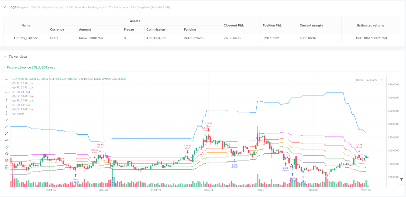
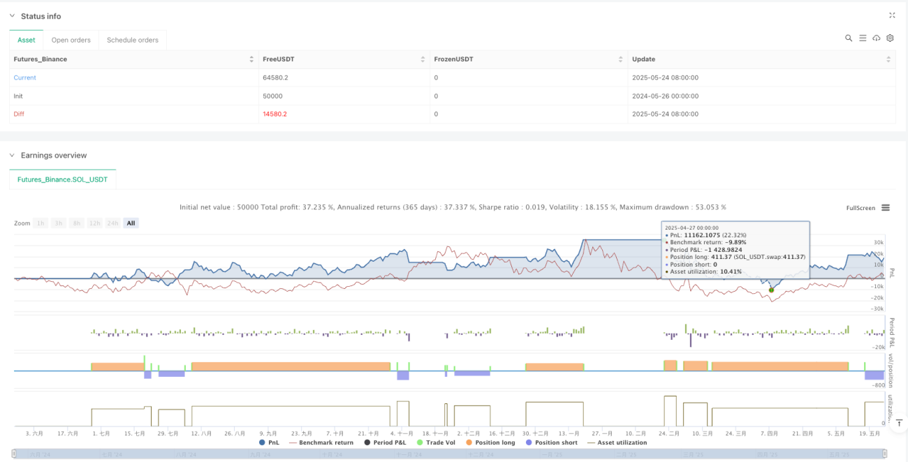
/*backtest
start: 2024-05-26 00:00:00
end: 2025-05-25 00:00:00
period: 2d
basePeriod: 2d
exchanges: [{"eid":"Futures_Binance","currency":"SOL_USDT"}]
*/

//@version=5
strategy("Fibonacci Trend v6.4 - TP/SL Labels", overlay=true, default_qty_type=strategy.percent_of_equity, default_qty_value=100)

// === Parameters ===
fibLen     = input.int(50, "Fibonacci Range")
fibTol     = input.float(0.01, "Fib Proximity Tolerance (%)", step=0.001)
slMult     = input.float(1.5, "SL - ATR", step=0.1)
tp2Mult    = input.float(2.0, "TP2 - ATR", step=0.1)
srLookback = input.int(20, "Support/Resistance Lookback Bars")
useBounce  = input.bool(true, "Enable Bounce Entry")

// === Indicators ===
ema50   = ta.ema(close, 50)
atr     = ta.atr(14)
volAvg  = ta.sma(volume, 20)
volHigh = volume > volAvg * 1.2

// === Fibonacci Levels ===
lowWick   = ta.lowest(low, fibLen)
highWick  = ta.highest(high, fibLen)
rangeWick = highWick - lowWick

fib236  = lowWick + 0.236 * rangeWick
fib382  = lowWick + 0.382 * rangeWick
fib5    = lowWick + 0.5   * rangeWick
fib618  = lowWick + 0.618 * rangeWick
fib786  = lowWick + 0.786 * rangeWick
fib1    = highWick
fib1618 = lowWick + 1.618 * rangeWick

nearSupport = math.abs(low - fib382)/close < fibTol or math.abs(low - fib5)/close < fibTol
nearResist  = math.abs(high - fib618)/close < fibTol

// === Trend Structure ===
higherLow   = low > low[1] and low[1] > low[2]
higherHigh  = high > high[1]
lowerHigh   = high < high[1] and high[1] < high[2]
lowerLow    = low < low[1]
longStruct  = higherLow and higherHigh
shortStruct = lowerHigh and lowerLow

// === ADX / DMI ===
dmiLen   = 14
upMove   = high - high[1]
downMove = low[1] - low
plusDM   = (upMove > downMove and upMove > 0) ? upMove : 0
minusDM  = (downMove > upMove and downMove > 0) ? downMove : 0
tr       = ta.tr(true)
tr14     = ta.rma(tr, dmiLen)
plusDI   = 100 * ta.rma(plusDM, dmiLen) / tr14
minusDI  = 100 * ta.rma(minusDM, dmiLen) / tr14
dx       = 100 * math.abs(plusDI - minusDI) / (plusDI + minusDI)
adx      = ta.rma(dx, dmiLen)
trendStrong = adx > 20

// === EMA Momentum Break ===
emaBreakLong  = close > ema50 and close[1] < ema50 and volume > volAvg
emaBreakShort = close < ema50 and close[1] > ema50 and volume > volAvg

// === Time Filter ===
var int lastLongBar = na
var int lastShortBar = na
canLong  = na(lastLongBar) or (bar_index - lastLongBar > 5)
canShort = na(lastShortBar) or (bar_index - lastShortBar > 5)

priceAboveEMA = close > ema50 and close[1] > ema50 and close[2] > ema50
priceBelowEMA = close < ema50 and close[1] < ema50 and close[2] < ema50

// === Support / Resistance ===
support = ta.lowest(low, srLookback)
resist  = ta.highest(high, srLookback)

// === Entry Conditions ===
longTrend  = priceAboveEMA and nearSupport and trendStrong and plusDI > minusDI and longStruct and (volHigh or emaBreakLong) and canLong
shortTrend = priceBelowEMA and nearResist  and trendStrong and minusDI > plusDI and shortStruct and (volHigh or emaBreakShort) and canShort

bounceLong  = useBounce and math.abs(low - support)/close < fibTol and close > open and close > close[1]
bounceShort = useBounce and math.abs(high - resist)/close < fibTol and close < open and close < close[1]

longSignal  = longTrend or bounceLong
shortSignal = shortTrend or bounceShort

// === TP/SL Calculations ===
tp1Long  = resist
tp2Long  = close + atr * tp2Mult
slLong   = close - atr * slMult

tp1Short = support
tp2Short = close - atr * tp2Mult
slShort  = close + atr * slMult

tp1ColorLong  = bounceLong  ? color.blue : color.yellow
tp1ColorShort = bounceShort ? color.blue : color.yellow

// === Long Entry ===
if (longSignal and strategy.position_size <= 0)
    strategy.entry("Long", strategy.long)
    strategy.exit("TP1", from_entry="Long", limit=tp1Long, stop=slLong, qty_percent=50)
    strategy.exit("TP2", from_entry="Long", limit=tp2Long, stop=slLong)
    lastLongBar := bar_index
    label.new(bar_index, close, text="ENTRY: " + str.tostring(close, "#.##"), style=label.style_label_down, color=color.green, textcolor=color.white)
    label.new(bar_index, tp1Long, text="TP1: " + str.tostring(tp1Long, "#.##"), style=label.style_label_down, color=tp1ColorLong)
    label.new(bar_index, tp2Long, text="TP2: " + str.tostring(tp2Long, "#.##"), style=label.style_label_down, color=color.green)
    label.new(bar_index, slLong,  text="SL: "  + str.tostring(slLong, "#.##"),  style=label.style_label_up, color=color.red)

// === Short Entry ===
if (shortSignal and strategy.position_size >= 0)
    strategy.entry("Short", strategy.short)
    strategy.exit("TP1", from_entry="Short", limit=tp1Short, stop=slShort, qty_percent=50)
    strategy.exit("TP2", from_entry="Short", limit=tp2Short, stop=slShort)
    lastShortBar := bar_index
    label.new(bar_index, close, text="ENTRY: " + str.tostring(close, "#.##"), style=label.style_label_up, color=color.red, textcolor=color.white)
    label.new(bar_index, tp1Short, text="TP1: " + str.tostring(tp1Short, "#.##"), style=label.style_label_up, color=tp1ColorShort)
    label.new(bar_index, tp2Short, text="TP2: " + str.tostring(tp2Short, "#.##"), style=label.style_label_up, color=color.green)
    label.new(bar_index, slShort,  text="SL: "  + str.tostring(slShort, "#.##"),  style=label.style_label_down, color=color.red)

// === Hedge Orders ===
if (strategy.position_size > 0 and shortSignal)
    strategy.entry("HedgeShort", strategy.short)

if (strategy.position_size < 0 and longSignal)
    strategy.entry("HedgeLong", strategy.long)

// === Fibonacci Plotting ===
plot(fib236,  "Fib 0.236",  color=color.gray)
plot(fib382,  "Fib 0.382",  color=color.green)
plot(fib5,    "Fib 0.5",    color=color.orange)
plot(fib618,  "Fib 0.618",  color=color.red)
plot(fib786,  "Fib 0.786",  color=color.fuchsia)
plot(fib1,    "Fib 1.0",    color=color.white)
plot(fib1618, "Fib 1.618",  color=color.blue)