The Kelly formula for positioning control of the lever

The Kelly formula for positioning control of the lever

** Assume stakes 1: Your probability of winning is 60%, the probability of losing is 40%; the net return on winning is 100%, and the loss on losing is 100%. This means that if you win, you can win $1 per bet, and if you lose, you will lose $1 per bet. The stakes can be made an infinite number of times, and each bet is arbitrarily set by you.

• 1, for this deadlock, the expected return on each bet is 60% * 1-40% * 1 = 20%, the expected return is positive.

  So how should we bet?

  If we don't think about it carefully, if we imagine roughly, we would think that since my expected return on each bet is 20%, in order to achieve the maximum return in the long run, I should try to put as much capital as possible into each bet.

  However, it is obviously unreasonable to put 100% of the capital into each round of gambling, because once a gambler loses, all the capital will be lost, and he will not be able to participate in the next round, only to leave the field.

  So the conclusion is that as long as there is a stalemate, the possibility of losing all the capital at once, even if it is very small, can never be filled. Because in the long run, small-probability events are inevitable, and in real life, the actual probability of small-probability events occurring is far greater than its theoretical probability. This is the fat tail effect in finance.

• 2, continue back to deadlock 1. Since it is unreasonable to bet 100% on every bet, what about 99%? If you bet 99% on every bet, you are not only guaranteed to never go broke, but you may even get a big return if you are lucky.

  Is this really what it looks like?

  Instead of analyzing the problem theoretically, we can do an experiment. We simulate the impasse and bet 99% each time to see what happens.

  The simulation experiment is very simple and can be done in Excel. See the diagram below:

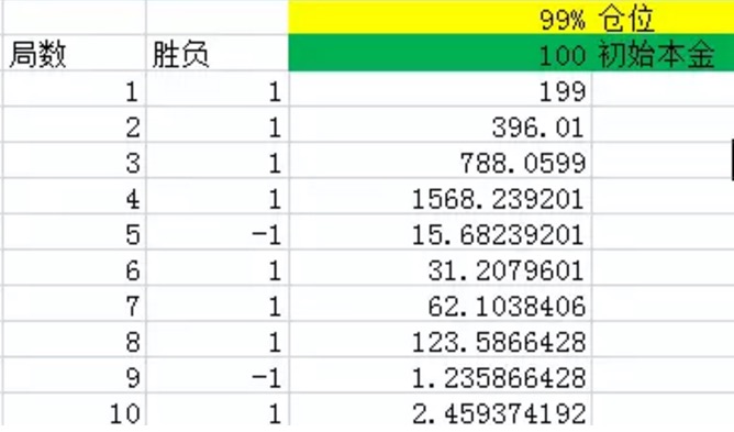  Figure 1

  As shown above, the first column represents the number of rounds; the second column is the win-loss, Excel will produce 1 with a 60% probability, or 60% probability, net return, with a 1.40% probability, or -1 with a 40% probability, net return. The third column is the total amount of money the bettor has at the end of each round.

  As you can see from the graph, after 10 rounds, the odds of winning in 10 rounds are 8 times greater than the 60% probability, losing only twice. But even so, the final amount is only 2.46 yuan, which is basically a loss.

  When I multiply the number of experiments by 1000, 2000, 3000... the result is that the final amount of money is basically going to zero.

  Since 99% doesn't work, let's try a few other ratios and see the graph below: It can be seen from the graph that when the position is gradually reduced, from 99%, to 90%, 80%, 70%, 60%, the result of the same 10 rounds is completely different. It seems that the money after 10 rounds is gradually increasing as the position gradually decreases.

  If you look at this, you will see that the problem of the stalemate is not so simple. Even with such a large stalemate, it is not easy to win.

  So how do you bet to maximize your long-term returns?

  Shouldn't it be, because obviously you can't make money when the ratio becomes zero?

  So what's the optimal ratio?

  This is the problem that the famous Kelly formula is trying to solve!

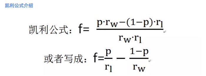  Figure 2

  where f is the optimal betting ratio; p is the probability of winning; rw is the net payoff when winning, e.g. rw=1 in tie-breaker 1; rl is the net loss when losing, e.g. rl=1 in tie-breaker 1; note here rl>0;

  According to Kelly's formula, the highest betting percentage in deadlock 1 can be calculated to be 20%.

  We can conduct an experiment to deepen our understanding of this conclusion.

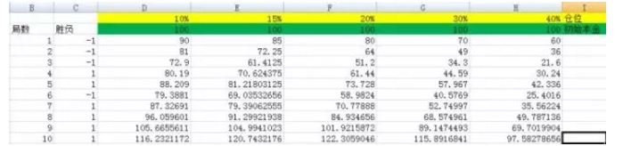  Figure 3

  In this example, we set the positions to 10%, 15%, 20%, 30%, 40% respectively. Their corresponding columns are D, E, F, G, H.

  When I converted the number of experiments to 3,000, When I converted the number of experiments to 5,000, You can see from this that the result of the F column corresponds to the largest, and the base is not a numerical scale compared to the other columns.

  Let's see the power of Kelly's formula. In the experiment above, if you unfortunately chose the proportion of 40%, which corresponds to column H, then after 5000 bets, your capital went from 100 to 22799985.75, a huge gain.

  This is the power of knowledge!

• Three, understanding the Kelly equation.

  The mathematical derivation of the Kelly equation and its complexity require a very high level of mathematical knowledge, so there is no point in discussing it here. Here I will deepen your understanding of the subjective nature of the Kelly equation through some experiments.

  Let's look at another deadlock. Deadlock 2: You have a 50% chance of winning and losing, for example, tossing a coin. The net return on winning is 1, which is rw = 1, and the net loss on losing is 0.5, which is rl = 0.5.

  It's easy to see that the expected return of the standoff 2 is 0.25, another standoff where the hackers have a huge advantage.

  According to Kelly's formula, we can get the optimal betting ratio per round:

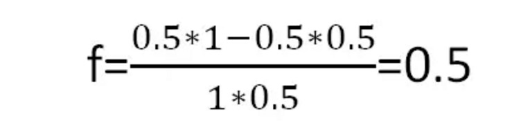  Figure four

  This means that every time you bet with half of your money, you get the maximum return in the long run.

  Here I will experimentally derive the concept of the average growth rate r.

  First, let's take a look at experiment 2.1, the following two diagrams:

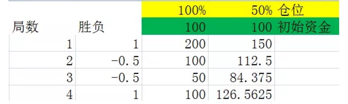  Figure 5

  The two graphs are simulations of a stalemate 2, in which the second column shows a 50% probability of a win, giving a profit of 100%. The 50% probability of a win, giving a loss of 50%. The third and fourth columns show the amount of money held after each stalemate at 100% and 50%, respectively.

  A careful comparison of the two diagrams leads to the conclusion that after the same number of rounds, the final result is only related to the number of rounds won and the number of rounds lost in these rounds, and not to the order of rounds won and rounds lost in these rounds. For example, in the first two diagrams, the same four rounds were done, and the same two rounds were lost in each diagram, but the order of the first graph is win-win-win-win, and the order of the second graph is win-win-win-win-win. They all end up the same.

  Of course, this conclusion is very easy to prove (the law of multiplication and substitution, elementary school students will), but it is not proven here, the two examples above are well enough to understand.

  So since the final outcome has nothing to do with the order in which you win or lose, we assume that deadlock 2 proceeds as experiment 2.2.

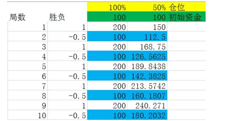  Figure 6

  We assume that the victories of the stalemate are alternated, and because of the conclusion one, this has no effect on the outcome funds in the long run.

  Before we look at the picture ourselves, we first make a definition. Suppose we consider a set of stalemates as a whole, in which the frequency of various outcomes is exactly equal to its probability, and the set of stalemates is the smallest of the set of stalemates in which all the conditions are met, then we call the set of stalemates a set of stalemates. For example, in the experiment shown above, a set of stalemates represents two stalemates in which one wins and one loses.

  Look closely at the numbers marked in blue in the diagram above, they are the end of a set of dead ends. You will find that the numbers are maintaining a steady growth. When the position is 100%, the growth rate of the blue marked numbers is 0%, i.e. the growth rate of the capital after a set of dead ends is 0%. This also explains why it is not possible to make money in the medium to long term in dead ends 2 when the positions are 50% (i.e. the optimal ratio derived by Kelly's formula), the growth rate of the blue marked numbers is 12.5%, i.e. the growth rate of the capital after a set of dead ends is 12.5%.

  It is a general law that the growth rate after each set of deadlocks is related to the position; and the higher the growth rate after each set of deadlocks, the greater the ultimate return in the long run.

  Based on the growth rate of each set of dead ends, the average growth rate of each dead end can be calculated g. In the figure above, if each set of dead ends contains two dead ends, then the average growth rate of each dead end is

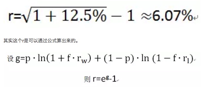  Figure 7

  In the long run, to maximize the growth of capital, we need to maximize r, i.e. maximize g. The optimal betting ratio f is also obtained by solving max (g).

• 4, Kelly's formula Other conclusions about risk

The Kelly Legend

Kelly's formula was originally created by AT&T Bell Laboratories physicist John Larry Kelly based on his colleague Claude Elwood Shannon's research on long-distance telephone lines. Kelly solved the problem of how Shannon's information theory should be applied to a gambler with intrinsic information at the time of the auction. The gambler wanted to decide the best bet amount, and his intrinsic information did not need to be perfect ("no information") to give him a useful advantage. Kelly's formula was later applied to twenty-one and the stock market by another of Shannon's colleagues, Edward Thorpe. Thorpe used his spare time and months of hard calculation to write a mathematical paper titled "The 21st Point Gambling Strategy". He used his knowledge to raid all the casinos in Reno, Nevada overnight and successfully win tens of thousands of dollars from the 21st Point Gambling Table. He is also the grandfather of the Wall Street Quantitative Trading Hedge Fund, and pioneered the first quantitative trading hedge fund in the 1970s.

Applying the prospect

How to make money in real life using Kelly's formula? That is to create a deadlock that satisfies the conditions for the application of the Kelly formula. Recently I have been doing research on trading systems, and what is most important for a good trading system? An expected return is 10% of the importance of positive buying and selling rules, while a good money control method is 40% of the importance, and the remaining 50% is the psychological control of manipulating people. The Kelly formula is exactly the tool that helped me control my money position. For example, a stock trading system I studied earlier, where the probability of a successful weekly trade is 0.8 and the probability of a failed weekly trade is 0.2; when successful, you can earn 3% (deduct commissions, stamp duty) and lose 5% on each failure. Before I knew the Kelly formula, I was a blind stockbroker, and I didn't know that the position setting was wrong, it was psychological. After using the Kelly formula, the best position to calculate should be 9.33, that is, if you want to get the fastest capital growth rate for a 0 interest rate leveraged trading, you need to calculate the average growth rate of leveraged trading per trade is about 7.44%, while the average capital growth rate of leveraged trading is about 1.35 (which is also the expected return). Of course, the Kelly formula cannot be as simple in practical application, and there are still many difficulties to overcome. For example, the cost of capital required for leveraged exchanges, for example, that money in reality is not infinitely divisible, for example, that in financial markets it is not as simple as the simple deadlock mentioned above. But in any case, Kelly's formula shows us the way forward.