CVD-Divergenz-quantitative Handelsstrategie

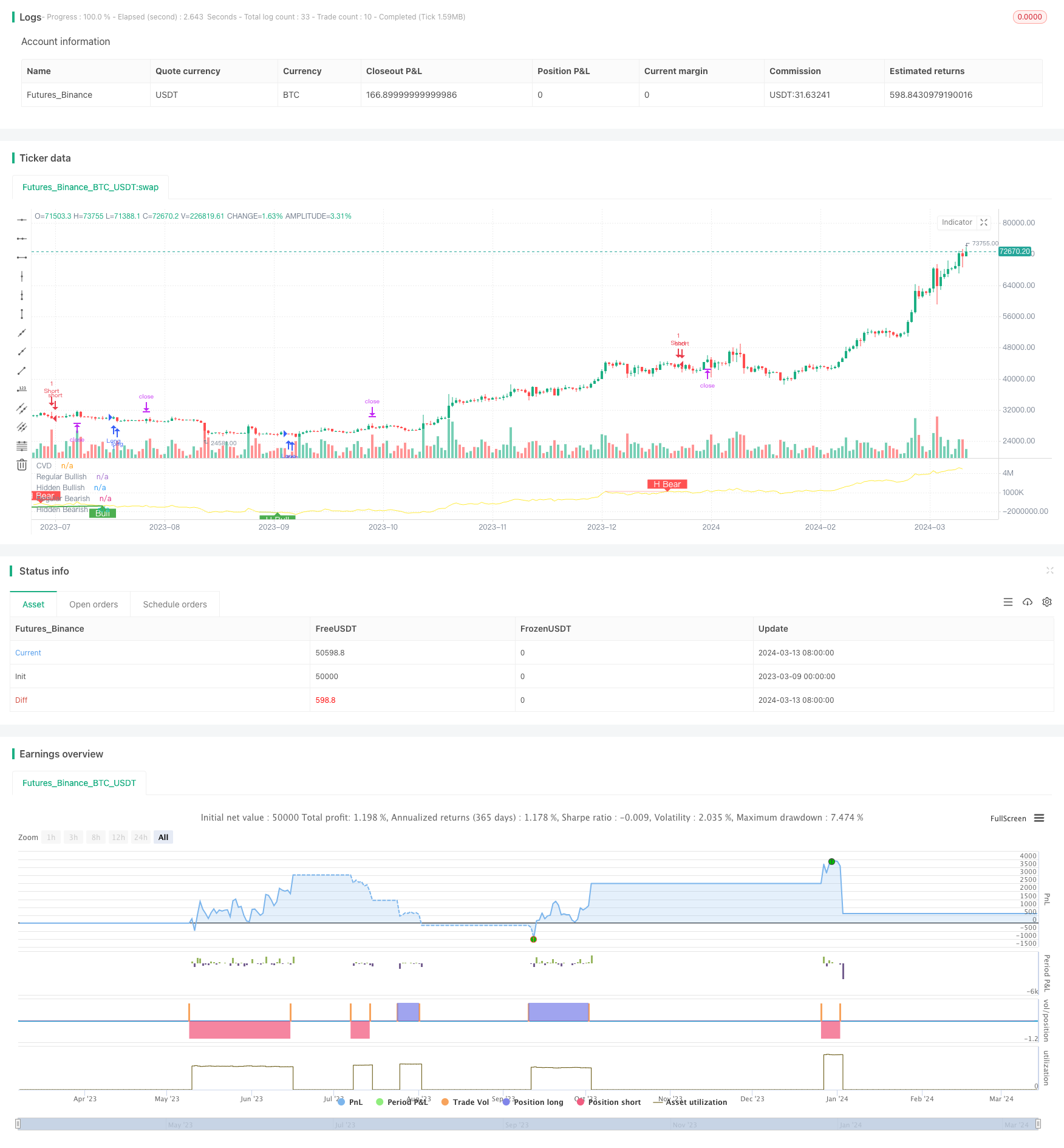
/*backtest
start: 2023-03-09 00:00:00
end: 2024-03-14 00:00:00
period: 1d
basePeriod: 1h
exchanges: [{"eid":"Futures_Binance","currency":"BTC_USDT"}]
*/

// This source code is subject to the terms of the Mozilla Public License 2.0 at https://mozilla.org/MPL/2.0/

//@version=5
//@ mmattman

//Thank you to @ contrerae and Tradingview each for parts of the code to make 
//this indicator and matching strategy and also theCrypster for the clean concise TP/SL code.

// indicator(title="CVD Divergence Indicator 1", shorttitle='CVD Div1', format=format.price, timeframe="", timeframe_gaps=true)

strategy("CVD Divergence Strategy.1.mm", shorttitle = 'CVD Div Str 1', overlay=false)


//..................................................................................................................
// Inputs
periodMa = input.int(title='MA Length', minval=1, defval=20)
plotMa = input(title='Plot MA?', defval=false)

// Calculations (Bull & Bear Balance Indicator by Vadim Gimelfarb)
iff_1 = close[1] < open ? math.max(high - close[1], close - low) : math.max(high - open, close - low)
iff_2 = close[1] > open ? high - low : math.max(open - close[1], high - low)
iff_3 = close[1] < open ? math.max(high - close[1], close - low) : high - open
iff_4 = close[1] > open ? high - low : math.max(open - close[1], high - low)
iff_5 = close[1] < open ? math.max(open - close[1], high - low) : high - low
iff_6 = close[1] > open ? math.max(high - open, close - low) : iff_5
iff_7 = high - close < close - low ? iff_4 : iff_6
iff_8 = high - close > close - low ? iff_3 : iff_7
iff_9 = close > open ? iff_2 : iff_8
bullPower = close < open ? iff_1 : iff_9
iff_10 = close[1] > open ? math.max(close[1] - open, high - low) : high - low
iff_11 = close[1] > open ? math.max(close[1] - low, high - close) : math.max(open - low, high - close)
iff_12 = close[1] > open ? math.max(close[1] - open, high - low) : high - low
iff_13 = close[1] > open ? math.max(close[1] - low, high - close) : open - low
iff_14 = close[1] < open ? math.max(open - low, high - close) : high - low
iff_15 = close[1] > open ? math.max(close[1] - open, high - low) : iff_14
iff_16 = high - close < close - low ? iff_13 : iff_15
iff_17 = high - close > close - low ? iff_12 : iff_16
iff_18 = close > open ? iff_11 : iff_17
bearPower = close < open ? iff_10 : iff_18

// Calculations (Bull & Bear Pressure Volume)
bullVolume = bullPower / (bullPower + bearPower) * volume
bearVolume = bearPower / (bullPower + bearPower) * volume

// Calculations Delta
delta = bullVolume - bearVolume
cvd = ta.cum(delta)
cvdMa = ta.sma(cvd, periodMa)

// Plotting
customColor = cvd > cvdMa ? color.new(color.teal, 50) : color.new(color.red, 50)
plotRef1 = plot(cvd, style=plot.style_line, linewidth=1, color=color.new(color.yellow, 0), title='CVD')
plotRef2 = plot(plotMa ? cvdMa : na, style=plot.style_line, linewidth=1, color=color.new(color.white, 0), title='CVD MA')
fill(plotRef1, plotRef2, color=customColor)
//..................................................................................................................


// len = input.int(title="RSI Period", minval=1, defval=14)
// src = input(title="RSI Source", defval=close)
lbR = input(title="Pivot Lookback Right", defval=3)
lbL = input(title="Pivot Lookback Left", defval=7)
rangeUpper = input(title="Max of Lookback Range", defval=60)
rangeLower = input(title="Min of Lookback Range", defval=5)
plotBull = input(title="Plot Bullish", defval=true)
plotHiddenBull = input(title="Plot Hidden Bullish", defval=true)
plotBear = input(title="Plot Bearish", defval=true)
plotHiddenBear = input(title="Plot Hidden Bearish", defval=true)
bearColor = color.red
bullColor = color.green
hiddenBullColor = color.new(color.green, 80)
hiddenBearColor = color.new(color.red, 80)
textColor = color.white
noneColor = color.new(color.white, 100)
osc = cvd

// plot(osc, title="CVD", linewidth=2, color=#2962FF)
// hline(50, title="Middle Line", color=#787B86, linestyle=hline.style_dotted)
// obLevel = hline(70, title="Overbought", color=#787B86, linestyle=hline.style_dotted)
// osLevel = hline(30, title="Oversold", color=#787B86, linestyle=hline.style_dotted)
// fill(obLevel, osLevel, title="Background", color=color.rgb(33, 150, 243, 90))

plFound = na(ta.pivotlow(osc, lbL, lbR)) ? false : true
phFound = na(ta.pivothigh(osc, lbL, lbR)) ? false : true
_inRange(cond) =>
	bars = ta.barssince(cond == true)
	rangeLower <= bars and bars <= rangeUpper

//------------------------------------------------------------------------------
// Regular Bullish
// Osc: Higher Low

oscHL = osc[lbR] > ta.valuewhen(plFound, osc[lbR], 1) and _inRange(plFound[1])

// Price: Lower Low

priceLL = low[lbR] < ta.valuewhen(plFound, low[lbR], 1)
bullCondAlert = priceLL and oscHL and plFound
bullCond = plotBull and bullCondAlert

plot(
     plFound ? osc[lbR] : na,
     offset=-lbR,
     title="Regular Bullish",
     linewidth=2,
     color=(bullCond ? bullColor : noneColor)
     )

plotshape(
	 bullCond ? osc[lbR] : na,
	 offset=-lbR,
	 title="Regular Bullish Label",
	 text=" Bull ",
	 style=shape.labelup,
	 location=location.absolute,
	 color=bullColor,
	 textcolor=textColor
	 )

//------------------------------------------------------------------------------
// Hidden Bullish
// Osc: Lower Low

oscLL = osc[lbR] < ta.valuewhen(plFound, osc[lbR], 1) and _inRange(plFound[1])

// Price: Higher Low

priceHL = low[lbR] > ta.valuewhen(plFound, low[lbR], 1)
hiddenBullCondAlert = priceHL and oscLL and plFound
hiddenBullCond = plotHiddenBull and hiddenBullCondAlert

plot(
	 plFound ? osc[lbR] : na,
	 offset=-lbR,
	 title="Hidden Bullish",
	 linewidth=2,
	 color=(hiddenBullCond ? hiddenBullColor : noneColor)
	 )

plotshape(
	 hiddenBullCond ? osc[lbR] : na,
	 offset=-lbR,
	 title="Hidden Bullish Label",
	 text=" H Bull ",
	 style=shape.labelup,
	 location=location.absolute,
	 color=bullColor,
	 textcolor=textColor
	 )

//------------------------------------------------------------------------------
// Regular Bearish
// Osc: Lower High

oscLH = osc[lbR] < ta.valuewhen(phFound, osc[lbR], 1) and _inRange(phFound[1])

// Price: Higher High

priceHH = high[lbR] > ta.valuewhen(phFound, high[lbR], 1)

bearCondAlert = priceHH and oscLH and phFound
bearCond = plotBear and bearCondAlert

plot(
	 phFound ? osc[lbR] : na,
	 offset=-lbR,
	 title="Regular Bearish",
	 linewidth=2,
	 color=(bearCond ? bearColor : noneColor)
	 )

plotshape(
	 bearCond ? osc[lbR] : na,
	 offset=-lbR,
	 title="Regular Bearish Label",
	 text=" Bear ",
	 style=shape.labeldown,
	 location=location.absolute,
	 color=bearColor,
	 textcolor=textColor
	 )

//------------------------------------------------------------------------------
// Hidden Bearish
// Osc: Higher High

oscHH = osc[lbR] > ta.valuewhen(phFound, osc[lbR], 1) and _inRange(phFound[1])

// Price: Lower High

priceLH = high[lbR] < ta.valuewhen(phFound, high[lbR], 1)

hiddenBearCondAlert = priceLH and oscHH and phFound
hiddenBearCond = plotHiddenBear and hiddenBearCondAlert

plot(
	 phFound ? osc[lbR] : na,
	 offset=-lbR,
	 title="Hidden Bearish",
	 linewidth=2,
	 color=(hiddenBearCond ? hiddenBearColor : noneColor)
	 )

plotshape(
	 hiddenBearCond ? osc[lbR] : na,
	 offset=-lbR,
	 title="Hidden Bearish Label",
	 text=" H Bear ",
	 style=shape.labeldown,
	 location=location.absolute,
	 color=bearColor,
	 textcolor=textColor
	 )

// alertcondition(bullCondAlert, title='Regular Bullish CVD Divergence', message="Found a new Regular Bullish Divergence, `Pivot Lookback Right` number of bars to the left of the current bar")
// alertcondition(hiddenBullCondAlert, title='Hidden Bullish CVD Divergence', message='Found a new Hidden Bullish Divergence, `Pivot Lookback Right` number of bars to the left of the current bar')
// alertcondition(bearCondAlert, title='Regular Bearish CVD Divergence', message='Found a new Regular Bearish Divergence, `Pivot Lookback Right` number of bars to the left of the current bar')
// alertcondition(hiddenBearCondAlert, title='Hidden Bearisn CVD Divergence', message='Found a new Hidden Bearisn Divergence, `Pivot Lookback Right` number of bars to the left of the current bar')

le = bullCondAlert or hiddenBullCondAlert

se = bearCondAlert or hiddenBearCondAlert

ltp = se

stp = le

// Check if the entry conditions for a long position are met
if (le) //and (close > ema200)
    strategy.entry("Long", strategy.long, comment="EL")

 // Check if the entry conditions for a short position are met
if (se) //and (close < ema200)
    strategy.entry("Short", strategy.short, comment="ES")

// Close long position if exit condition is met
if (ltp) // or (close < ema200)
    strategy.close("Long", comment="XL")

    // Close short position if exit condition is met
if (stp) //or (close > ema200)
    strategy.close("Short", comment="XS")


// The Fixed Percent Stop Loss Code
// User Options to Change Inputs (%)
stopPer = input.float(5.0, title='Stop Loss %') / 100
takePer = input.float(10.0, title='Take Profit %') / 100

// Determine where you've entered and in what direction
longStop = strategy.position_avg_price * (1 - stopPer)
shortStop = strategy.position_avg_price * (1 + stopPer)
shortTake = strategy.position_avg_price * (1 - takePer)
longTake = strategy.position_avg_price * (1 + takePer)

if strategy.position_size > 0 
    strategy.exit("Close Long", "Long", stop=longStop, limit=longTake)
if strategy.position_size < 0 
    strategy.exit("Close Short", "Short", stop=shortStop, limit=shortTake)