Estrategia de negociación cuantitativa de divergencia CVD
Resumen de la estrategia: La estrategia de comercio cuantitativo de desviación de CVD utiliza el indicador de CVD y la desviación de la formación del precio para capturar una señal de cambio de tendencia potencial. La estrategia calcula los indicadores de CVD y, al compararlos con el precio, determina si se forma una desviación alcista o bajista.
Principio de la estrategia:
- Calculación del indicador CVD: Calcula el indicador CVD y sus medias móviles en función del volumen de transacciones de más y de menos.
- Identificar desviaciones: determinar si se han formado desviaciones comparando los puntos altos y bajos de los indicadores de CVD con los puntos altos y bajos de los precios.
- Desviación de la tendencia habitual: la innovación en precios es baja, pero los indicadores de CVD se forman en puntos más altos y más bajos
- Los precios de la innovación son altos, pero el indicador de CVD forma bajos más bajos
- Desviación de la tendencia bajista habitual: los precios crean altos, pero el indicador CVD forma altos más bajos
- La baja oculta de los bajistas: la innovación en los precios es baja, pero los indicadores de CVD forman un punto más alto
- Abrir posiciones: cuando se reconoce una señal de desviación, abrir posiciones en exceso o en blanco según el tipo de desviación.
- Stop loss: se utiliza el stop loss móvil y el stop loss porcentual fijo. El precio de stop loss se calcula en función del precio de apertura multiplicado por el porcentaje de stop loss, y el precio de stop loss se calcula en función del precio de apertura multiplicado por el porcentaje de stop loss.
- Incremento de la pirámide: la estrategia permite un incremento de la pirámide de hasta 3 posiciones.
Las ventajas estratégicas:
- Señales de cambio de tendencia: La desviación de CVD es una señal de cambio de tendencia eficaz que puede ayudar a capturar oportunidades de cambio de tendencia.
- Señales de continuación de la tendencia: La desviación oculta puede servir como señal de continuación de la tendencia, ayudando a la estrategia a mantener la dirección correcta en la tendencia.
- Control de riesgo: El uso de stop loss móvil y stop loss de porcentaje fijo permite un control efectivo del riesgo.
- La pirámide de subida de posiciones: permite subidas de posiciones en muchas posiciones para aprovechar mejor las tendencias.
El riesgo estratégico:
- Eficacia de la señal: La desviación de la señal no es totalmente confiable, a veces se produce una falsa señal.
- Configuración de parámetros: los resultados de la estrategia son sensibles a la configuración de parámetros, y diferentes parámetros pueden producir diferentes resultados.
- Punto de pérdida: en situaciones extremas, las órdenes de pérdida pueden no ser negociadas al precio predeterminado, lo que conlleva un riesgo adicional.
- Gastos de transacción: La apertura frecuente de posiciones cerradas puede generar altos costos de transacción y afectar los beneficios de la estrategia.
La dirección de la optimización:
- Optimización de parámetros dinámicos: Parámetros adaptados a las diferentes condiciones del mercado para mejorar la eficacia de la señal.
- Combinación con otros indicadores: Combinación con otros indicadores técnicos como RSI, MACD, etc., para mejorar la fiabilidad de la señal.
- Mejorar el stop loss: adopta estrategias de stop loss más avanzadas, como el seguimiento de los stops, los stops de fluctuación, etc.
- Gestión del tamaño de la posición: ajuste el tamaño de la posición en función de la volatilidad del mercado, el capital de la cuenta y otros factores.
En resumen: La estrategia de CVD deviation quantitative trading captura el desvío de los indicadores de CVD con respecto al precio y identifica las oportunidades potenciales de reversión de la tendencia. Al mismo tiempo, utiliza un stop loss móvil y un porcentaje fijo de control de stop loss. La principal ventaja de la estrategia es que puede capturar de manera efectiva las señales de reversión de tendencia y la continuación de la tendencia, y controlar mejor la situación de la tendencia a través de la pirámide. Sin embargo, la estrategia también presenta riesgos como la eficacia de la señal, la configuración de parámetros, los puntos de deslizamiento de stop loss y los costos de transacción.
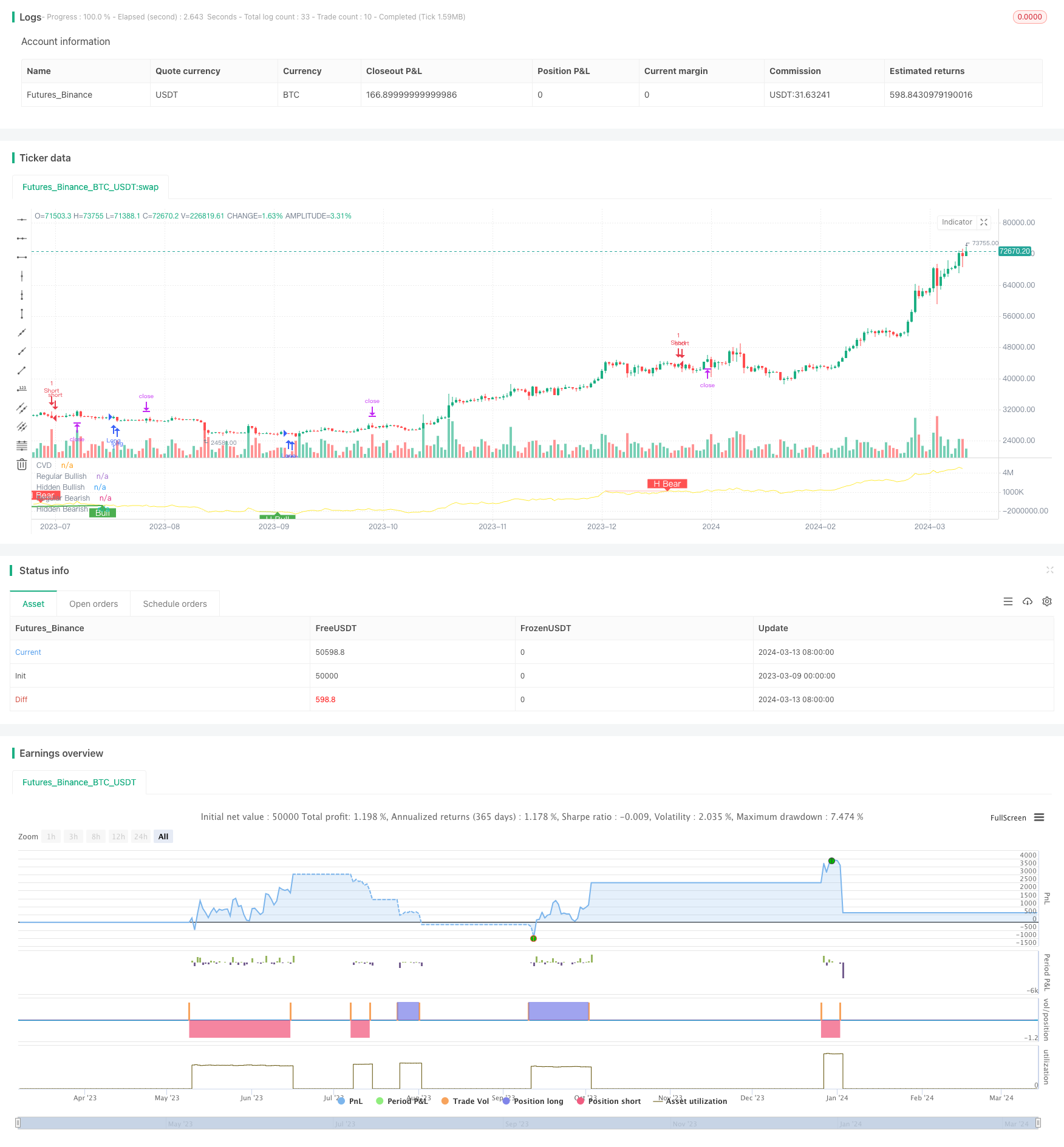
/*backtest
start: 2023-03-09 00:00:00
end: 2024-03-14 00:00:00
period: 1d
basePeriod: 1h
exchanges: [{"eid":"Futures_Binance","currency":"BTC_USDT"}]
*/

// This source code is subject to the terms of the Mozilla Public License 2.0 at https://mozilla.org/MPL/2.0/

//@version=5
//@ mmattman

//Thank you to @ contrerae and Tradingview each for parts of the code to make
//this indicator and matching strategy and also theCrypster for the clean concise TP/SL code.

// indicator(title="CVD Divergence Indicator 1", shorttitle='CVD Div1', format=format.price, timeframe="", timeframe_gaps=true)

strategy("CVD Divergence Strategy.1.mm", shorttitle = 'CVD Div Str 1', overlay=false)


//..................................................................................................................
// Inputs
periodMa = input.int(title='MA Length', minval=1, defval=20)
plotMa = input(title='Plot MA?', defval=false)

// Calculations (Bull & Bear Balance Indicator by Vadim Gimelfarb)
iff_1 = close[1] < open ? math.max(high - close[1], close - low) : math.max(high - open, close - low)
iff_2 = close[1] > open ? high - low : math.max(open - close[1], high - low)
iff_3 = close[1] < open ? math.max(high - close[1], close - low) : high - open
iff_4 = close[1] > open ? high - low : math.max(open - close[1], high - low)
iff_5 = close[1] < open ? math.max(open - close[1], high - low) : high - low
iff_6 = close[1] > open ? math.max(high - open, close - low) : iff_5
iff_7 = high - close < close - low ? iff_4 : iff_6
iff_8 = high - close > close - low ? iff_3 : iff_7
iff_9 = close > open ? iff_2 : iff_8
bullPower = close < open ? iff_1 : iff_9
iff_10 = close[1] > open ? math.max(close[1] - open, high - low) : high - low
iff_11 = close[1] > open ? math.max(close[1] - low, high - close) : math.max(open - low, high - close)
iff_12 = close[1] > open ? math.max(close[1] - open, high - low) : high - low
iff_13 = close[1] > open ? math.max(close[1] - low, high - close) : open - low
iff_14 = close[1] < open ? math.max(open - low, high - close) : high - low
iff_15 = close[1] > open ? math.max(close[1] - open, high - low) : iff_14
iff_16 = high - close < close - low ? iff_13 : iff_15
iff_17 = high - close > close - low ? iff_12 : iff_16
iff_18 = close > open ? iff_11 : iff_17
bearPower = close < open ? iff_10 : iff_18

// Calculations (Bull & Bear Pressure Volume)
bullVolume = bullPower / (bullPower + bearPower) * volume
bearVolume = bearPower / (bullPower + bearPower) * volume

// Calculations Delta
delta = bullVolume - bearVolume
cvd = ta.cum(delta)
cvdMa = ta.sma(cvd, periodMa)

// Plotting
customColor = cvd > cvdMa ? color.new(color.teal, 50) : color.new(color.red, 50)
plotRef1 = plot(cvd, style=plot.style_line, linewidth=1, color=color.new(color.yellow, 0), title='CVD')
plotRef2 = plot(plotMa ? cvdMa : na, style=plot.style_line, linewidth=1, color=color.new(color.white, 0), title='CVD MA')
fill(plotRef1, plotRef2, color=customColor)
//..................................................................................................................


// len = input.int(title="RSI Period", minval=1, defval=14)
// src = input(title="RSI Source", defval=close)
lbR = input(title="Pivot Lookback Right", defval=3)
lbL = input(title="Pivot Lookback Left", defval=7)
rangeUpper = input(title="Max of Lookback Range", defval=60)
rangeLower = input(title="Min of Lookback Range", defval=5)
plotBull = input(title="Plot Bullish", defval=true)
plotHiddenBull = input(title="Plot Hidden Bullish", defval=true)
plotBear = input(title="Plot Bearish", defval=true)
plotHiddenBear = input(title="Plot Hidden Bearish", defval=true)
bearColor = color.red
bullColor = color.green
hiddenBullColor = color.new(color.green, 80)
hiddenBearColor = color.new(color.red, 80)
textColor = color.white
noneColor = color.new(color.white, 100)
osc = cvd

// plot(osc, title="CVD", linewidth=2, color=#2962FF)
// hline(50, title="Middle Line", color=#787B86, linestyle=hline.style_dotted)
// obLevel = hline(70, title="Overbought", color=#787B86, linestyle=hline.style_dotted)
// osLevel = hline(30, title="Oversold", color=#787B86, linestyle=hline.style_dotted)
// fill(obLevel, osLevel, title="Background", color=color.rgb(33, 150, 243, 90))

plFound = na(ta.pivotlow(osc, lbL, lbR)) ? false : true
phFound = na(ta.pivothigh(osc, lbL, lbR)) ? false : true
_inRange(cond) =>
	bars = ta.barssince(cond == true)
	rangeLower <= bars and bars <= rangeUpper

//------------------------------------------------------------------------------
// Regular Bullish
// Osc: Higher Low

oscHL = osc[lbR] > ta.valuewhen(plFound, osc[lbR], 1) and _inRange(plFound[1])

// Price: Lower Low

priceLL = low[lbR] < ta.valuewhen(plFound, low[lbR], 1)
bullCondAlert = priceLL and oscHL and plFound
bullCond = plotBull and bullCondAlert

plot(
     plFound ? osc[lbR] : na,
     offset=-lbR,
     title="Regular Bullish",
     linewidth=2,
     color=(bullCond ? bullColor : noneColor)
     )

plotshape(
	 bullCond ? osc[lbR] : na,
	 offset=-lbR,
	 title="Regular Bullish Label",
	 text=" Bull ",
	 style=shape.labelup,
	 location=location.absolute,
	 color=bullColor,
	 textcolor=textColor
	 )

//------------------------------------------------------------------------------
// Hidden Bullish
// Osc: Lower Low

oscLL = osc[lbR] < ta.valuewhen(plFound, osc[lbR], 1) and _inRange(plFound[1])

// Price: Higher Low

priceHL = low[lbR] > ta.valuewhen(plFound, low[lbR], 1)
hiddenBullCondAlert = priceHL and oscLL and plFound
hiddenBullCond = plotHiddenBull and hiddenBullCondAlert

plot(
	 plFound ? osc[lbR] : na,
	 offset=-lbR,
	 title="Hidden Bullish",
	 linewidth=2,
	 color=(hiddenBullCond ? hiddenBullColor : noneColor)
	 )

plotshape(
	 hiddenBullCond ? osc[lbR] : na,
	 offset=-lbR,
	 title="Hidden Bullish Label",
	 text=" H Bull ",
	 style=shape.labelup,
	 location=location.absolute,
	 color=bullColor,
	 textcolor=textColor
	 )

//------------------------------------------------------------------------------
// Regular Bearish
// Osc: Lower High

oscLH = osc[lbR] < ta.valuewhen(phFound, osc[lbR], 1) and _inRange(phFound[1])

// Price: Higher High

priceHH = high[lbR] > ta.valuewhen(phFound, high[lbR], 1)

bearCondAlert = priceHH and oscLH and phFound
bearCond = plotBear and bearCondAlert

plot(
	 phFound ? osc[lbR] : na,
	 offset=-lbR,
	 title="Regular Bearish",
	 linewidth=2,
	 color=(bearCond ? bearColor : noneColor)
	 )

plotshape(
	 bearCond ? osc[lbR] : na,
	 offset=-lbR,
	 title="Regular Bearish Label",
	 text=" Bear ",
	 style=shape.labeldown,
	 location=location.absolute,
	 color=bearColor,
	 textcolor=textColor
	 )

//------------------------------------------------------------------------------
// Hidden Bearish
// Osc: Higher High

oscHH = osc[lbR] > ta.valuewhen(phFound, osc[lbR], 1) and _inRange(phFound[1])

// Price: Lower High

priceLH = high[lbR] < ta.valuewhen(phFound, high[lbR], 1)

hiddenBearCondAlert = priceLH and oscHH and phFound
hiddenBearCond = plotHiddenBear and hiddenBearCondAlert

plot(
	 phFound ? osc[lbR] : na,
	 offset=-lbR,
	 title="Hidden Bearish",
	 linewidth=2,
	 color=(hiddenBearCond ? hiddenBearColor : noneColor)
	 )

plotshape(
	 hiddenBearCond ? osc[lbR] : na,
	 offset=-lbR,
	 title="Hidden Bearish Label",
	 text=" H Bear ",
	 style=shape.labeldown,
	 location=location.absolute,
	 color=bearColor,
	 textcolor=textColor
	 )

// alertcondition(bullCondAlert, title='Regular Bullish CVD Divergence', message="Found a new Regular Bullish Divergence, `Pivot Lookback Right` number of bars to the left of the current bar")
// alertcondition(hiddenBullCondAlert, title='Hidden Bullish CVD Divergence', message='Found a new Hidden Bullish Divergence, `Pivot Lookback Right` number of bars to the left of the current bar')
// alertcondition(bearCondAlert, title='Regular Bearish CVD Divergence', message='Found a new Regular Bearish Divergence, `Pivot Lookback Right` number of bars to the left of the current bar')
// alertcondition(hiddenBearCondAlert, title='Hidden Bearisn CVD Divergence', message='Found a new Hidden Bearisn Divergence, `Pivot Lookback Right` number of bars to the left of the current bar')

le = bullCondAlert or hiddenBullCondAlert

se = bearCondAlert or hiddenBearCondAlert

ltp = se

stp = le

// Check if the entry conditions for a long position are met
if (le) //and (close > ema200)
    strategy.entry("Long", strategy.long, comment="EL")

 // Check if the entry conditions for a short position are met
if (se) //and (close < ema200)
    strategy.entry("Short", strategy.short, comment="ES")

// Close long position if exit condition is met
if (ltp) // or (close < ema200)
    strategy.close("Long", comment="XL")

    // Close short position if exit condition is met
if (stp) //or (close > ema200)
    strategy.close("Short", comment="XS")


// The Fixed Percent Stop Loss Code
// User Options to Change Inputs (%)
stopPer = input.float(5.0, title='Stop Loss %') / 100
takePer = input.float(10.0, title='Take Profit %') / 100

// Determine where you've entered and in what direction
longStop = strategy.position_avg_price * (1 - stopPer)
shortStop = strategy.position_avg_price * (1 + stopPer)
shortTake = strategy.position_avg_price * (1 - takePer)
longTake = strategy.position_avg_price * (1 + takePer)

if strategy.position_size > 0
    strategy.exit("Close Long", "Long", stop=longStop, limit=longTake)
if strategy.position_size < 0
    strategy.exit("Close Short", "Short", stop=shortStop, limit=shortTake)