Chiến lược giao dịch đảo ngược đường trung bình động


Ngày tạo: 2023-10-26 15:38:14 sửa đổi lần cuối: 2023-10-26 15:38:14
sao chép: 0 Số nhấp chuột: 628
1
tập trung vào
1617
Người theo dõi

Chiến lược giao dịch đảo ngược đường trung bình động

Tổng quan

Chiến lược giao dịch quay trở lại đường trung bình là một chiến lược giao dịch dựa trên mức độ lệch của giá từ đường trung bình. Chiến lược này sử dụng các đặc điểm của giá lệch ngắn hạn từ đường trung bình dài hạn, thiết lập vị trí khi giá thấp hơn hoặc cao hơn đường trung bình đáng kể và tháo lỗ khi giá quay trở lại đường trung bình.

Nguyên tắc chiến lược

Chiến lược này đầu tiên tính toán trung bình di chuyển trong một chu kỳ, đại diện cho xu hướng giá dài hạn. Sau đó, thời gian và quy mô vị trí được xác định dựa trên mức độ lệch của giá so với trung bình di chuyển.

Khi giá thấp hơn một tỷ lệ nhất định so với đường trung bình di chuyển, đại diện cho giá lệch khỏi xu hướng dài hạn, khi đó theo tỷ lệ vị trí nhất định, nhiều đơn vị được thành lập dần dần. Càng giá lệch càng nhiều, vị trí được thành lập càng lớn. Khi giá tăng trở lại cao hơn đường trung bình di chuyển, đại diện cho sự trở lại xu hướng dài hạn, khi đó theo tỷ lệ vị trí.

Tương tự như vậy, khi giá cao hơn một tỷ lệ nhất định so với trung bình di chuyển, đặt lệnh trống. Khi giá giảm trở lại trung bình di chuyển, cân bằng tỷ lệ.

Phân tích lợi thế

  1. Sử dụng khả năng nhận dạng xu hướng của đường trung bình, theo xu hướng cân bằng dài hạn của giá cổ phiếu, nắm bắt hướng xu hướng chính.

  2. Xây dựng vị thế theo lô, giảm chi phí xây dựng kho và có được giá chi phí tốt hơn.

  3. Sử dụng ngưng ngưng từng giai đoạn, mức độ quay trở lại khác nhau có cơ hội ngưng ngưng khác nhau, giảm nguy cơ.

  4. Kiểm soát vị thế sử dụng phần cố định để tránh tổn thất đơn lẻ quá lớn.

  5. Cài đặt tham số linh hoạt, có thể điều chỉnh theo chu kỳ trung bình di chuyển hoặc tỷ lệ vị trí tùy theo giống khác nhau.

Phân tích rủi ro

  1. Khi giá dao động, có thể dừng lại thường xuyên. Có thể nới lỏng mức dừng lại thích hợp, hoặc sử dụng các điều kiện lọc khác.

  2. Các cổ phiếu mạnh có thể phá vỡ đường trung bình và tiếp tục tăng hoặc giảm, không thể quay trở lại điểm dừng trung bình. Các chỉ số xu hướng có thể kết hợp để xác định xu hướng mạnh và giảm vị thế.

  3. Thiết lập tham số không đúng có thể dẫn đến việc đặt cược hoặc dừng lỗ quá mạnh. Các tham số nên được thử nghiệm cẩn thận và điều chỉnh theo thị trường.

  4. Chi phí giao dịch có thể cao hơn khi giao dịch thường xuyên, nên xem xét các tham số tối ưu hóa yếu tố chi phí.

Hướng tối ưu hóa

  1. Tối ưu hóa chu kỳ trung bình di chuyển để thích ứng với các đặc điểm khác nhau của giống.

  2. Tối ưu hóa tỷ lệ vị thế, cân bằng rủi ro lợi nhuận.

  3. Thêm bộ lọc các chỉ số kỹ thuật khác để tránh giao dịch không cần thiết.

  4. Kết hợp với chỉ số biến động, điều chỉnh tỷ lệ vị trí theo mức độ biến động của thị trường.

  5. Tham gia vào cơ chế tăng cường, giảm rủi ro, tăng lợi nhuận.

Tóm tắt

Chiến lược quay trở lại đường trung bình sử dụng tính năng quay trở lại cân bằng của cổ phiếu, đặt vị trí khi giá lệch khỏi đường trung bình di chuyển, dừng lại khi giá quay trở lại, có thể nắm bắt hiệu quả xu hướng dài hạn của cổ phiếu. Bằng cách tối ưu hóa tham số và lọc chỉ số, có thể thích ứng với sự thay đổi của thị trường, thu được lợi nhuận tốt hơn với điều kiện kiểm soát rủi ro. Chiến lược này xem xét theo dõi xu hướng và tập trung vào kiểm soát rủi ro, đáng để các nhà đầu tư nghiên cứu và áp dụng.
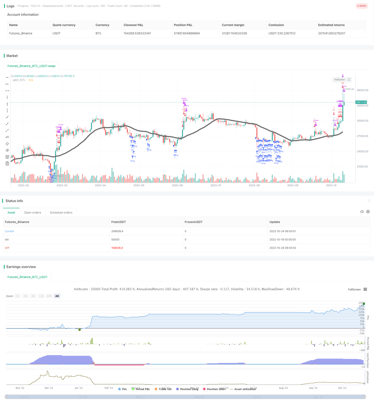
Mã nguồn chiến lược
/*backtest
start: 2022-10-19 00:00:00
end: 2023-10-25 00:00:00
period: 1d
basePeriod: 1h
exchanges: [{"eid":"Futures_Binance","currency":"BTC_USDT"}]
*/

//@version=4
strategy("YJ Mean Reversion", overlay=true)
//Was designed firstly to work on an index like the S&P 500 , which over time tends to go up in value. 
//Avoid trading too frequently (e.g. Daily, Weekly), to avoid getting eaten by fees. 
//If you change the underlying asset, or time frame, tweaking the moving average may be necessary. 
//Can work with a starting capital of just $1000, optimise the settings as necessary. 
//Accepts floating point values for the amount of units to purchase (e.g. Bitcoin ). 
//If price of units exceeds available capital, script will cancel the buy. 
//Adjusted the input parameters to be more intuitive.

//input variables
movingAverage = input(title="Moving Average (bars)", type=input.integer, defval=28, minval=1, maxval=1000)
//riskPercentage = input(title="Amount to Risk (%)", type=input.integer, defval=1, minval=1, maxval=50)
deviation = input(title="Deviation Increment (%)", type=input.float, defval=5, minval=0.01, maxval=100) / 100
unitsLevel1 = input(title="Level 1 (units)", type=input.float, defval=1, minval=0.0001, maxval=10000)
unitsLevel2 = input(title="Level 2 (units)", type=input.float, defval=2, minval=0.0001, maxval=10000)
unitsLevel3 = input(title="Level 3 (units)", type=input.float, defval=4, minval=0.0001, maxval=10000)
unitsLevel4 = input(title="Level 4 (units)", type=input.float, defval=8, minval=0.0001, maxval=10000)
unitsLevel5 = input(title="Level 5 (units)", type=input.float, defval=16, minval=0.0001, maxval=10000)

//moving average and ma slope (use on weekly chart)
ma = sma(close, movingAverage)
//sl = ma > ma[4]

//units to buy
//amount = riskPercentage / 100 * (strategy.initial_capital + strategy.netprofit)
//units = floor(amount / close)

//mode 1
//strategy.order("buy", true, 1, when = (close < 0.95 * ma) and (strategy.position_size < 10))
//strategy.order("sell", false, strategy.position_size, when = (close > 1.05 * ma) and (strategy.position_size > 0))

//mode 2
//strategy.order("buy", true, 1, when = close < 0.8 * ma)
//strategy.order("sell", false, strategy.position_size, when = (close > 310) and (strategy.position_size > 0))

//mode 3
//strategy.order("buy", true, 1, when = (close < 0.95 * ma) and (close > 0.9 * ma))
//strategy.order("buy", true, 2, when = (close < 0.9 * ma) and (close > 0.85 * ma))
//strategy.order("buy", true, 4, when = (close < 0.85 * ma) and (close > 0.8 * ma))
//strategy.order("buy", true, 8, when = (close < 0.8 * ma) and (close > 0.75 * ma))
//strategy.order("buy", true, 16, when = (close < 0.75 * ma))
//strategy.order("sell", false, strategy.position_size, when = (close > 310) and (strategy.position_size > 0))

//mode 4
//strategy.order("buy", true, 1, when = (close < 0.98 * ma) and (close > 0.96 * ma) and (sl))
//strategy.order("buy", true, 2, when = (close < 0.96 * ma) and (close > 0.94 * ma) and (sl))
//strategy.order("buy", true, 4, when = (close < 0.94 * ma) and (close > 0.92 * ma) and (sl))
//strategy.order("buy", true, 8, when = (close < 0.92 * ma) and (close > 0.90 * ma) and (sl))
//strategy.order("buy", true, 16, when = (close < 0.90 * ma) and (sl))
//strategy.order("sell", false, strategy.position_size, when = (close > 310) and (strategy.position_size > 0))

//mode 5
//strategy.order("buy", true, 1, when = (close < 0.95 * ma) and (close > 0.9 * ma))
//strategy.order("buy", true, 2, when = (close < 0.9 * ma) and (close > 0.85 * ma))
//strategy.order("buy", true, 4, when = (close < 0.85 * ma) and (close > 0.8 * ma))
//strategy.order("buy", true, 8, when = (close < 0.8 * ma) and (close > 0.75 * ma))
//strategy.order("buy", true, 16, when = (close < 0.75 * ma))

//strategy.order("sell", false, 1, when = (close > 1.05 * ma) and (close < 1.1 * ma) and (strategy.position_size > 0))
//strategy.order("sell", false, 2, when = (close > 1.1 * ma) and (close < 1.15 * ma) and (strategy.position_size > 0))
//strategy.order("sell", false, 4, when = (close > 1.15 * ma) and (close < 1.2 * ma) and (strategy.position_size > 0))
//strategy.order("sell", false, 8, when = (close > 1.2 * ma) and (close < 1.25 * ma) and (strategy.position_size > 0))
//strategy.order("sell", false, 16, when = (close > 1.25 * ma) and (close < 1.3 * ma) and (strategy.position_size > 0))

//mode 6
//strategy.order("B1", true, unitsLevel1 * units, when = (close < 0.95 * ma) and (close > 0.9 * ma))
//strategy.order("B2", true, unitsLevel2 * units, when = (close < 0.9 * ma) and (close > 0.85 * ma))
//strategy.order("B3", true, unitsLevel3 * units, when = (close < 0.85 * ma) and (close > 0.8 * ma))
//strategy.order("B4", true, unitsLevel4 * units, when = (close < 0.8 * ma) and (close > 0.75 * ma))
//strategy.order("B5", true, unitsLevel5 * units, when = (close < 0.75 * ma))

//strategy.order("S1", false, unitsLevel1 * units, when = (close > 1.05 * ma) and (close < 1.1 * ma) and (strategy.position_size > 0))
//strategy.order("S2", false, unitsLevel2 * units, when = (close > 1.1 * ma) and (close < 1.15 * ma) and (strategy.position_size > 0))
//strategy.order("S3", false, unitsLevel3 * units, when = (close > 1.15 * ma) and (close < 1.2 * ma) and (strategy.position_size > 0))
//strategy.order("S4", false, unitsLevel4 * units, when = (close > 1.2 * ma) and (close < 1.25 * ma) and (strategy.position_size > 0))
//strategy.order("S5", false, unitsLevel5 * units, when = (close > 1.25 * ma) and (close < 1.3 * ma) and (strategy.position_size > 0))

//mode 7
//strategy.order("B1", true, units, when = (close < 0.95 * ma) and (close > 0.9 * ma))
//strategy.order("B2", true, units, when = (close < 0.9 * ma) and (close > 0.85 * ma))
//strategy.order("B3", true, units, when = (close < 0.85 * ma) and (close > 0.8 * ma))
//strategy.order("B4", true, units, when = (close < 0.8 * ma) and (close > 0.75 * ma))
//strategy.order("B5", true, units, when = (close < 0.75 * ma))

//strategy.order("S1", false, units, when = (close > 1.05 * ma) and (close < 1.1 * ma) and (strategy.position_size > 0))
//strategy.order("S2", false, units, when = (close > 1.1 * ma) and (close < 1.15 * ma) and (strategy.position_size > 0))
//strategy.order("S3", false, units, when = (close > 1.15 * ma) and (close < 1.2 * ma) and (strategy.position_size > 0))
//strategy.order("S4", false, units, when = (close > 1.2 * ma) and (close < 1.25 * ma) and (strategy.position_size > 0))
//strategy.order("S5", false, units, when = (close > 1.25 * ma) and (close < 1.3 * ma) and (strategy.position_size > 0))

//banding calculations
aH = 1.0 - deviation
aL = aH - deviation
bH = aL
bL = bH - deviation
cH = bL
cL = cH - deviation
dH = cL
dL = dH - deviation
eH = dL
strategy.initial_capital = 50000
//mode 8
strategy.order("B1", true, unitsLevel1, when = (close < aH * ma) and (close > aL * ma) and (unitsLevel1 * close < (strategy.initial_capital + strategy.netprofit)))
strategy.order("B2", true, unitsLevel2, when = (close < bH * ma) and (close > bL * ma) and (unitsLevel2 * close < (strategy.initial_capital + strategy.netprofit)))
strategy.order("B3", true, unitsLevel3, when = (close < cH * ma) and (close > cL * ma) and (unitsLevel3 * close < (strategy.initial_capital + strategy.netprofit)))
strategy.order("B4", true, unitsLevel4, when = (close < dH * ma) and (close > dL * ma) and (unitsLevel4 * close < (strategy.initial_capital + strategy.netprofit)))
strategy.order("B5", true, unitsLevel5, when = (close < eH * ma) and (unitsLevel5 * close < (strategy.initial_capital + strategy.netprofit)))

//banding calculations
fL = 1.0 + deviation
fH = fL + deviation
gL = fH
gH = gL + deviation
hL = gH
hH = hL + deviation
iL = hH
iH = iL + deviation
jL = iH

strategy.order("S1", false, unitsLevel1, when = (close > fL * ma) and (close < fH * ma) and (strategy.position_size > 0))
strategy.order("S2", false, unitsLevel2, when = (close > gL * ma) and (close < gH * ma) and (strategy.position_size > 0))
strategy.order("S3", false, unitsLevel3, when = (close > hL * ma) and (close < hH * ma) and (strategy.position_size > 0))
strategy.order("S4", false, unitsLevel4, when = (close > iL * ma) and (close < iH * ma) and (strategy.position_size > 0))
strategy.order("S5", false, unitsLevel5, when = (close > jL * ma) and (strategy.position_size > 0))

plot(ma, color=#666666, linewidth=5)