Multifaktorielle adaptive Momentum-Tracking-Strategie


Erstellungsdatum: 2023-12-12 12:02:13 zuletzt geändert: 2023-12-12 12:02:13
Kopie: 0 Klicks: 648
1
konzentrieren Sie sich auf
1621
Anhänger

Multifaktorielle adaptive Momentum-Tracking-Strategie

Überblick

Die Multi-Faktor Adaptive Dynamics Tracking Strategie ermöglicht den automatisierten Handel mit hochflüchtigen Vermögenswerten wie Kryptowährungen durch die Integration mehrerer technischer Indikatoren zur Identifizierung von Markttrends und wichtigen Unterstützungswiderstände. Die Strategie nutzt Indicatoren wie den RSI, MACD und Stochastic, um Kauf- und Verkaufsmomente zu bestimmen, und kombiniert diese mit dem Prozentsatz der Preisänderung, um eine genauere Form zu identifizieren.

Strategieprinzip

Der Kern der Multifaktor-Adaptive-Dynamik-Tracking-Strategie liegt in der integrierten Anwendung mehrerer technischer Indikatoren. Die Strategie verwendet hauptsächlich die folgenden Komponenten:

  1. Der RSI-Indikator beurteilt Überkaufe und Überverkäufe. In Kombination mit verschiedenen Parametern kann ein normales RSI-Signal oder eine verbesserte Version des Conner-RSI-Signals erkannt werden, um zu beurteilen, ob eine Umkehrmöglichkeit besteht.

  2. Der MACD-Indikator hilft bei der Bestimmung der Trendrichtung. Es erzeugt Kauf- und Verkaufssignale, wenn der MACD die Signallinie auf- oder abläuft.

  3. Der Stochastic-Indikator identifiziert Überkauf-Überverkaufszonen. Die K- und D-Linien des Gold-Stock-Stock-Kombinationssignals beurteilen, ob sie umgekehrt sind.

  4. Der Prozentsatz der Preisänderung prüft, ob es sich um einen echten Durchbruch handelt. Der Prozentsatz der Veränderung des Höchstpreises, des Tiefpreises, des Schlusspreises usw. in einem bestimmten Zeitraum wird berechnet, um zu beurteilen, ob es sich um einen echten Durchbruch handelt.

  5. EMA-Indikatoren beurteilen die hohe Bandbreite. Überschreiten Sie die schnelle Linie als bullish Signal, und überschreiten Sie die langsame Linie als bearish Signal.

Die Strategie basiert auf der Wahl, mehr zu machen, wenn der Markt leer ist, und setzt eine Stop-Loss-Stopp-Lösung, um das Risiko effektiv zu kontrollieren. Wenn ein Umkehrsignal auftritt, wählt man einen Ausgang aus der Position. Der gesamte Entscheidungsprozess ist in vollem Umfang mit mehreren Faktoren verbunden, um eine genauere Entscheidung zu erzielen.

Analyse der Stärken

Die Strategie hat folgende Vorteile:

  1. Mehrfaktoren haben einen entscheidenden Vorteil. Im Vergleich zu einzelnen Indikatoren können Kombinationen von mehreren Indikatoren gegenseitig verifiziert werden, wodurch die Ergebnisse genauer und zuverlässiger sind und unnötige Transaktionskosten eingespart werden.

  2. Die Strategie setzt strenge Anforderungen an die Kauf- und Verkaufskonditionen, die mehrere Indikatoren erfordern, um gleichzeitig Signale freizusetzen, um eine Menge Geräusche zu filtern und falsche Geschäfte zu vermeiden.

  3. Die Fähigkeit, die Parameter der Strategie dynamisch zu berechnen, um die Subjektivität der manuellen Auswahl der Hyperparameter zu vermeiden, wodurch die Strategie-Parameter wissenschaftlicher objektiv gemacht werden.

  4. Die Strategie berechnet und zeichnet die Stop-Loss-Stop-Position in Echtzeit nach der Positionseröffnung aus, um Einzelschäden effektiv zu kontrollieren und die Entstehung von Ausbrüchen zu vermeiden.

Risikoanalyse

Die Strategie birgt auch einige Risiken, die zu vermeiden sind:

  1. Die Wahrscheinlichkeit, dass ein Indikator fehlsignalisiert wird. Obwohl die Multi-Indikator-Verifizierung die Fehlsignalrate erheblich reduzieren kann, ist es immer noch möglich, dass dies geschieht. Dies kann zu unnötigen Verlusten führen.

  2. Das Risiko, dass der Stop-Loss durchbrochen wird. In extremen Situationen kann es zu einem Absturz des Preises kommen, der dazu führt, dass der ursprüngliche Stop-Loss leicht durchbrochen wird, was zu einem größeren Verlust führt.

  3. Überoptimierung durch Parameteroptimierung. Dynamische Parameter vermeiden zwar die Subjektivität einer künstlichen Auswahl, können aber auch dazu führen, dass Parameter überoptimiert werden und ihre Allgemeinerungsfähigkeit verloren gehen.

Entsprechende Lösungen:

  1. Erhöhen Sie die Strenge der Signalfilterbedingungen und reduzieren Sie die Fehlsignalrate.
  2. Die Einrichtung der Lagerhalle in Schüttungen verhindert, dass ein einziger Schaden zu groß wird.
  3. Erhöhung der Probenmenge und strenge Bewertung der Parameterstabilität.

Richtung der Strategieoptimierung

Es gibt mehrere Optimierungsdimensionen für die Multi-Factor Adaptive Dynamic Tracking Strategie:

  1. Erhöhung der Anzahl von Urteilsfaktoren. Zusätzliche Urteile in Verbindung mit mehr verschiedenen Arten von Indikatorsignal-Urteilen wie Volatilität, Handelsvolumen usw.

  2. Optimierung von Stop-Loss-Algorithmen. Es können fortschrittlichere Stop-Loss-Algorithmen wie Tracking-Stop, Shake-Stop eingeführt werden, um die Wahrscheinlichkeit, dass die Stop-Loss-Systeme durchbrochen werden, weiter zu reduzieren.

  3. Einführung von Machine Learning-Modellen. Modelle wie RNN, LSTM und andere werden verwendet, um historische Daten zu modellieren, um Kauf- und Verkaufsentscheidungen zu treffen.

  4. Strategieintegration. Die Integration von mehreren Unterstrategien mit Hilfe von integrierten Lernmethoden kann zu einer stabileren Gesamtleistung führen.

Zusammenfassen

Die Integration von mehreren technischen Indikatoren zur Identifizierung von Kauf- und Verkaufszeiten. Die Strategie ist genauer als ein einzelner Indikator, während die eingebauten Parameter die Risiken der Selbstanpassung und der Stop-Loss-Mechanismen kontrollieren. Der nächste Schritt besteht darin, die Wirksamkeit der Strategie durch die Einführung von zusätzlichen Hilfsentscheidungsfaktoren, fortschrittlichen Stop-Loss-Algorithmen und Methoden wie Machine Learning weiter zu verbessern.
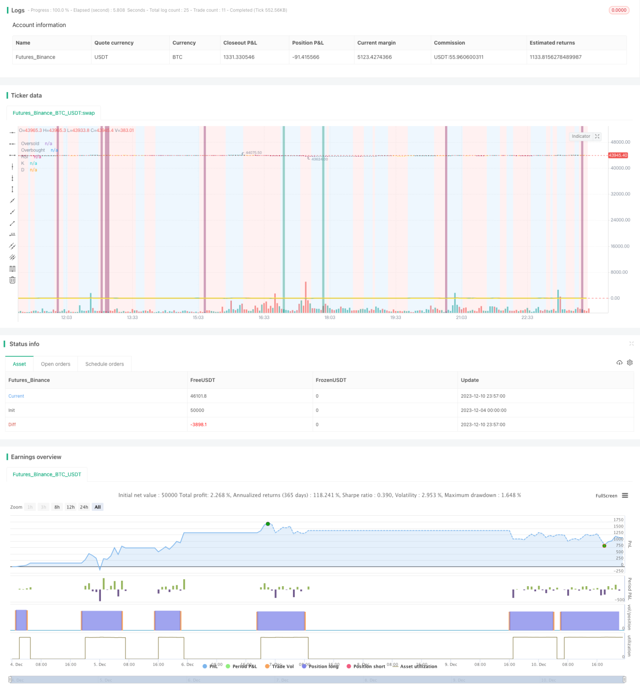
Strategiequellcode
/*backtest
start: 2023-12-04 00:00:00
end: 2023-12-11 00:00:00
period: 3m
basePeriod: 1m
exchanges: [{"eid":"Futures_Binance","currency":"BTC_USDT"}]
*/

// This source code is subject to the terms of the Mozilla Public License 2.0 at https://mozilla.org/MPL/2.0/
//@version=4

// ██████╗██████╗ ███████╗ █████╗ ████████╗███████╗██████╗     ██████╗ ██╗   ██╗    
//██╔════╝██╔══██╗██╔════╝██╔══██╗╚══██╔══╝██╔════╝██╔══██╗    ██╔══██╗╚██╗ ██╔╝                       
//██║     ██████╔╝█████╗  ███████║   ██║   █████╗  ██║  ██║    ██████╔╝ ╚████╔╝                        
//██║     ██╔══██╗██╔══╝  ██╔══██║   ██║   ██╔══╝  ██║  ██║    ██╔══██╗  ╚██╔╝                         
//╚██████╗██║  ██║███████╗██║  ██║   ██║   ███████╗██████╔╝    ██████╔╝   ██║                          
// ╚═════╝╚═╝  ╚═╝╚══════╝╚═╝  ╚═╝   ╚═╝   ╚══════╝╚═════╝     ╚═════╝    ╚═╝                          
                                                                                                     
//███████╗ ██████╗ ██╗     ██╗   ██╗████████╗██╗ ██████╗ ███╗   ██╗███████╗ ██╗ █████╗ ███████╗ █████╗ 
//██╔════╝██╔═══██╗██║     ██║   ██║╚══██╔══╝██║██╔═══██╗████╗  ██║██╔════╝███║██╔══██╗╚════██║██╔══██╗
//███████╗██║   ██║██║     ██║   ██║   ██║   ██║██║   ██║██╔██╗ ██║███████╗╚██║╚██████║    ██╔╝╚█████╔╝
//╚════██║██║   ██║██║     ██║   ██║   ██║   ██║██║   ██║██║╚██╗██║╚════██║ ██║ ╚═══██║   ██╔╝ ██╔══██╗
//███████║╚██████╔╝███████╗╚██████╔╝   ██║   ██║╚██████╔╝██║ ╚████║███████║ ██║ █████╔╝   ██║  ╚█████╔╝
//╚══════╝ ╚═════╝ ╚══════╝ ╚═════╝    ╚═╝   ╚═╝ ╚═════╝ ╚═╝  ╚═══╝╚══════╝ ╚═╝ ╚════╝    ╚═╝   ╚════╝ 

strategy(shorttitle='Ain1 No Label',title='All in One Strategy no RSI Label', overlay=true, scale=scale.left, initial_capital = 1000, process_orders_on_close=true, default_qty_type = strategy.percent_of_equity, default_qty_value = 100, commission_type=strategy.commission.percent, commission_value=0.18, calc_on_every_tick=true)

kcolor = color.new(#0094FF, 60)
dcolor = color.new(#FF6A00, 60)


// -----------------  Strategy Inputs -------------------------------------------------------------
//Backtest dates with auto finish date of today
start = input(defval = timestamp("01 April 2021 00:00 -0500"), title = "Start Time", type = input.time)
finish = input(defval = timestamp("31 December 2021 00:00 -0600"), title = "End Time", type = input.time)
window()  => true       // create function "within window of time"


// Strategy Selection - Long, Short, or Both
stratinfo = input(true, "Long/Short for Mixed Market, Long for Bull, Short for Bear")
strat = input(title="Trade Types", defval="Long/Short", options=["Long Only", "Long/Short", "Short Only"])
strat_val = strat == "Long Only" ? 1 : strat == "Long/Short" ? 0 : -1

// Risk Management Inputs
sl= input(10.0, "Stop Loss %", minval = 0, maxval = 100, step = 0.01)
stoploss = sl/100
tp = input(20.0, "Target Profit %", minval = 0, maxval = 100, step = 0.01)
TargetProfit = tp/100


useXRSI = input(false, "Use RSI crossing back, select only one strategy")
useCRSI = input(false, "Use Tweaked Connors RSI, select only one")
RSIInfo = input(true, "These are the RSI Strategy Inputs, RSI Length applies to MACD, set OB and OS to 45 for using Stoch and EMA strategies.")
length = input(14, "RSI Length", minval=1)
overbought= input(62, "Overbought")
oversold= input(35, "Oversold")
cl1 = input(3, "Connor's MA Length 1", minval=1, step=1)
cl2 = input(20, "Connor's MA Lenght 2", minval=1, step=1)
cl3 = input(50, "Connor's MA Lenght 3", minval=1, step=1)

// MACD and EMA Inputs
useMACD = input(false, "Use MACD Only, select only one strategy")
useEMA  = input(false, "Use EMA Only, select only one strategy (EMA uses Stochastic inputs too)")
MACDInfo=input(true, "These are the MACD strategy variables")
fastLength = input(5, minval=1, title="EMA Fast Length")
slowLength = input(10, minval=1, title="EMA Slow Length")
ob_min = input(52, "Overbought Lookback Minimum Value", minval=0, maxval=200)
ob_lb = input(25, "Overbought Lookback Bars", minval=0, maxval=100)
os_min = input(50, "Oversold Lookback Minimum Value", minval=0, maxval=200)
os_lb = input(35, "Oversold Lookback Bars", minval=0, maxval=100)
source = input(title="Source", type=input.source, defval=close)
RSI = rsi(source, length)


// Price Movement Inputs
PriceInfo = input(true, "Price Change Percentage Cross Check Inputs for all Strategies, added logic to avoid early sell")
lkbk = input(5,"Max Lookback Period")

// EMA and SMA Background Inputs
useStoch    = input(false, "Use Stochastic Strategy, choose only one")
StochInfo   = input(true, "Stochastic Strategy Inputs")
smoothK     = input(3, "K", minval=1)
smoothD     = input(3, "D", minval=1)
k_mode      = input("SMA", "K Mode", options=["SMA", "EMA", "WMA"])
high_source = input(high,"High Source")
low_source= input(low,"Low Source")
HTF = input("","Curernt or Higher time frame only", type=input.resolution)

// Selections to show or hide the overlays
showZones = input(true, title="Show Bullish/Bearish Zones")
showStoch = input(true, title="Show Stochastic Overlays")
showRSIBS = input(true, title="Show RSI Buy Sell Zones")
showMACD = input(true, title="Show MACD")
color_bars=input(true, "Color Bars")


// ------------------ Dynamic RSI Calculation ----------------------------------------

AvgHigh(src,cnt,val) =>
    total = 0.0
    count = 0
    for i = 0 to cnt
        if src[i] > val
            count := count + 1
            total := total + src[i]
    round(total / count)
    
RSI_high = AvgHigh(RSI, ob_lb, ob_min)

AvgLow(src,cnt,val) =>
    total = 0.0
    count = 0
    for i = 0 to cnt
        if src[i] < val
            count := count + 1
            total := total + src[i]
    round(total / count)

RSI_low = AvgLow(RSI, os_lb, os_min)


// ------------------ Price Percentage Change Calculation -----------------------------------------
perc_change(lkbk) =>
    overall_change = ((close[0] - open[lkbk]) / open[lkbk]) * 100
    highest_high = 0.0
    lowest_low = 0.0
    for i = lkbk to 0
        highest_high := i == lkbk ? high : high[i] > high[(i + 1)] ? high[i] : highest_high[1]
        lowest_low := i == lkbk ? low : low[i] < low[(i + 1)] ? low[i] : lowest_low[1]
    
    start_to_high = ((highest_high - open[lkbk]) / open[lkbk]) * 100
    start_to_low = ((lowest_low - open[lkbk]) / open[lkbk]) * 100
    previous_to_high = ((highest_high - open[1])/open[1])*100
    previous_to_low = ((lowest_low-open[1])/open[1])*100
    previous_bar = ((close[1]-open[1])/open[1])*100
    
    [overall_change, start_to_high, start_to_low, previous_to_high, previous_to_low, previous_bar]
    
// Call the function    
[overall, to_high, to_low, last_high, last_low, last_bar] = perc_change(lkbk)

// Plot the function
//plot(overall*50, color=color.white, title='Overall Percentage Change', linewidth=3)
//plot(to_high*50, color=color.green,title='Percentage Change from Start to High', linewidth=2)
//plot(to_low*50, color=color.red, title='Percentage Change from Start to Low', linewidth=2)
//plot(last_high*100, color=color.teal, title="Previous to High", linewidth=2)
//plot(last_low*100, color=color.maroon, title="Previous to Close", linewidth=2)
//plot(last_bar*100, color=color.orange, title="Previous Bar", linewidth=2)
//hline(0, title='Center Line', color=color.orange, linewidth=2)

true_dip = overall < 0 and to_high > 0 and to_low < 0 and last_high > 0 and last_low < 0 and last_bar < 0
true_peak = overall > 0 and to_high > 0 and to_low > 0 and last_high > 0 and last_low < 0 and last_bar > 0

alertcondition(true_dip, title='True Dip', message='Dip')
alertcondition(true_peak, title='True Peak', message='Peak')

// ------------------ Background Colors based on EMA Indicators -----------------------------------
// Uses standard lengths of 9 and 21, if you want control delete the constant definition and uncomment the inputs
haClose(gap) => (open[gap] + high[gap] + low[gap] + close[gap]) / 4
rsi_ema = rsi(haClose(0), length)
v2 = ema(rsi_ema, length)                                                
v3 = 2 * v2 - ema(v2, length)  
emaA = ema(rsi_ema, fastLength)                                     
emaFast = 2 * emaA - ema(emaA, fastLength)
emaB = ema(rsi_ema, slowLength)                                     
emaSlow = 2 * emaB - ema(emaB, slowLength) 

//plot(rsi_ema, color=color.white, title='RSI EMA', linewidth=3)
//plot(v2, color=color.green,title='v2', linewidth=2)
//plot(v3, color=color.red, title='v3', linewidth=2)
//plot(emaFast, color=color.teal, title="EMA Fast", linewidth=2)
//plot(emaSlow, color=color.maroon, title="EMA Slow", linewidth=2)

EMABuy = crossunder(emaFast, v2) and window()
EMASell = crossover(emaFast, emaSlow) and window()


alertcondition(EMABuy, title='EMA Buy', message='EMA Buy Condition')
alertcondition(EMASell, title='EMA Sell', message='EMA Sell Condition')


// bullish signal rule: 
bullishRule =emaFast > emaSlow
// bearish signal rule: 
bearishRule =emaFast < emaSlow

// current trading State
ruleState = 0
ruleState := bullishRule ? 1 : bearishRule ? -1 : nz(ruleState[1])
ruleColor = ruleState==1 ? color.new(color.blue, 90) : ruleState == -1 ? color.new(color.red, 90) : ruleState == 0 ? color.new(color.gray, 90) : na
bgcolor(showZones ? ruleColor : na, title="Bullish/Bearish Zones")


// ------------------  Stochastic Indicator Overlay -----------------------------------------------

// Calculation
// Use highest highs and lowest lows
h_high = highest(high_source ,lkbk)
l_low = lowest(low_source ,lkbk)

stoch = stoch(RSI, RSI_high, RSI_low, length)
k =
 k_mode=="EMA" ? ema(stoch, smoothK) :
 k_mode=="WMA" ? wma(stoch, smoothK) :
 sma(stoch, smoothK)
d = sma(k, smoothD)
k_c = change(k)
d_c = change(d)
kd = k - d

// Plot
signalColor = k>oversold and d<overbought and k>d and k_c>0 and d_c>0 ? kcolor : 
 k<overbought and d>oversold and k<d and k_c<0 and d_c<0 ? dcolor : na
kp = plot(showStoch ? k : na, "K", color=kcolor)
dp = plot(showStoch ? d : na, "D", color=dcolor)
fill(kp, dp, color = signalColor, title="K-D")
signalUp = showStoch ? not na(signalColor) and kd>0 : na
signalDown = showStoch ? not na(signalColor) and kd<0 : na
//plot(signalUp ? kd : na, "Signal Up", color=kcolor, transp=90, style=plot.style_columns)
//plot(signalDown ? (kd+100) : na , "Signal Down", color=dcolor, transp=90, style=plot.style_columns, histbase=100)

//StochBuy = crossover(k, d) and kd>0 and to_low<0 and window()
//StochSell = crossunder(k,d) and kd<0 and to_high>0 and window()

StochBuy = crossover(k, d) and window()
StochSell = crossunder(k, d) and window()

alertcondition(StochBuy, title='Stoch Buy', message='K Crossing D')
alertcondition(StochSell, title='Stoch Sell', message='D Crossing K')


// -------------- Add Price Movement -------------------------
// Calculations
h1 = vwma(high, length)
l1 = vwma(low, length)
hp = h_high[1]
lp = l_low[1]

// Plot
var plot_color=#353535
var sig = 0
if (h1 >hp)
    sig:=1
    plot_color:=color.lime
else if (l1 <lp)
    sig:=-1
    plot_color:=color.maroon
//plot(1,title = "Price Movement Bars", style=plot.style_columns,color=plot_color)
//plot(sig,title="Signal 1 or -1",display=display.none)


// --------------------------------------- RSI Plot ----------------------------------------------
// Plot Oversold and Overbought Lines
over = hline(oversold, title="Oversold", color=color.green)
under = hline(overbought, title="Overbought", color=color.red)
fillcolor = color.new(#9915FF, 90)
fill(over, under, fillcolor, title="Band Background")


// Show RSI and EMA crosses with arrows and RSI Color (tweaked Connors RSI)
// Improves strategy setting ease by showing where EMA 5 crosses EMA 10 from above to confirm overbought conditions or trend reversals
// This shows where you should enter shorts or exit longs

// Tweaked Connors RSI Calculation
connor_ob = overbought
connor_os = oversold
ma1 = sma(close,cl1)
ma2 = sma(close, cl2)
ma3 = sma(close, cl3)

// Buy Sell Zones using tweaked Connors RSI (RSI values of 80 and 20 for Crypto as well as ma3, ma20, and ma50 are the tweaks)
RSI_SELL = ma1 > ma2 and open > ma3 and RSI >= connor_ob and true_peak and window()
RSI_BUY = ma2 < ma3 and ma3 > close and RSI <= connor_os and true_dip and window()

alertcondition(RSI_BUY, title='Connors Buy', message='Connors RSI Buy')
alertcondition(RSI_SELL, title='Connors Sell', message='Connors RSI Sell')

// Color Definition
col = useCRSI ? (close > ma2 and close < ma3 and RSI <= connor_os ? color.lime : close < ma2 and close > ma3 and RSI <= connor_ob ? color.red : color.yellow ) : color.yellow

// Plot colored RSI Line
plot(RSI, title="RSI", linewidth=3, color=col)


//------------------- MACD Strategy -------------------------------------------------
[macdLine, signalLine, _] = macd(close, fastLength, slowLength, length)

bartrendcolor = macdLine > signalLine and k > 50 and RSI > 50 ? color.teal : macdLine < signalLine and k < 50 and RSI < 50 ? color.maroon : macdLine < signalLine ? color.yellow : color.gray
barcolor(color = color_bars ? bartrendcolor : na)


MACDBuy = macdLine>signalLine and RSI<RSI_low and overall<0 and window()
MACDSell = macdLine<signalLine and RSI>RSI_high and overall>0 and window()

//plotshape(showMACD ? MACDBuy: na, title = "MACD Buy", style = shape.arrowup, text = "MACD Buy", color=color.green, textcolor=color.green, size=size.small)
//plotshape(showMACD ? MACDSell: na, title = "MACD Sell", style = shape.arrowdown, text = "MACD Sell", color=color.red, textcolor=color.red, size=size.small)
MACColor = MACDBuy ? color.new(color.teal, 50) : MACDSell ? color.new(color.maroon, 50) : na
bgcolor(showMACD ? MACColor : na, title ="MACD Signals")


// -------------------------------- Entry and Exit Logic ------------------------------------


// Entry Logic
XRSI_OB = crossunder(RSI, overbought) and overall<0 and window()
RSI_OB = RSI>overbought and true_peak and window()
XRSI_OS = crossover(RSI, oversold) and overall>0 and window()
RSI_OS = RSI<oversold and true_dip and window()

alertcondition(XRSI_OB, title='Reverse RSI Sell', message='RSI Crossing back under OB')
alertcondition(XRSI_OS, title='Reverse RSI Buy', message='RSI Crossing back over OS')

alertcondition(RSI_OS, title='RSI Buy', message='RSI Crossover OS')
alertcondition(RSI_SELL, title='RSI Sell', message='RSI Crossunder OB')


// Strategy Entry and Exit with built in Risk Management
GoLong = strategy.position_size==0 and strat_val > -1 and rsi_ema > RSI and k < d ? (useXRSI ? XRSI_OS : useMACD ? MACDBuy : useCRSI ? RSI_BUY : useStoch ? StochBuy : RSI_OS) : false

GoShort = strategy.position_size==0 and strat_val < 1 and rsi_ema < RSI and d < k ? (useXRSI ? XRSI_OB : useMACD ? MACDSell : useCRSI ? RSI_SELL : useStoch ? StochSell : RSI_OB) : false

if (GoLong)
    strategy.entry("LONG", strategy.long)

if (GoShort) 
    strategy.entry("SHORT", strategy.short)


longStopPrice  = strategy.position_avg_price * (1 - stoploss)
longTakePrice  = strategy.position_avg_price * (1 + TargetProfit)
shortStopPrice = strategy.position_avg_price * (1 + stoploss)
shortTakePrice = strategy.position_avg_price * (1 - TargetProfit)

//plot(series=(strategy.position_size > 0) ? longTakePrice : na, color=color.green, style=plot.style_circles, linewidth=3, title="Long Take Profit")
//plot(series=(strategy.position_size < 0) ? shortTakePrice : na, color=color.green, style=plot.style_circles, linewidth=3, title="Short Take Profit")
//plot(series=(strategy.position_size > 0) ? longStopPrice : na, color=color.red, style=plot.style_cross, linewidth=2, title="Long Stop Loss")
//plot(series=(strategy.position_size < 0) ? shortStopPrice : na, color=color.red, style=plot.style_cross, linewidth=2, title="Short Stop Loss")

if (strategy.position_size > 0)
    strategy.exit(id="Exit Long", from_entry = "LONG", stop = longStopPrice, limit = longTakePrice)
    
if (strategy.position_size < 0)
    strategy.exit(id="Exit Short", from_entry = "SHORT", stop = shortStopPrice, limit = shortTakePrice)


CloseLong = strat_val > -1 and strategy.position_size > 0 and rsi_ema > RSI and d > k ? (useXRSI ? XRSI_OB : useMACD ? MACDSell : useCRSI ? RSI_SELL : RSI_OB) : false

if(CloseLong)
    strategy.close("LONG")
        
CloseShort = strat_val < 1 and strategy.position_size < 0 and rsi_ema < RSI and k > d ? (useXRSI ? XRSI_OS : useMACD ? MACDBuy : useCRSI ? RSI_BUY : RSI_OS) : false

if(CloseShort)
    strategy.close("SHORT")