Estrategia de seguimiento de tendencias de filtros de doble alcance

El autor:¿ Qué pasa?, Fecha: 2024-02-05 11:15:28
Las etiquetas:

Resumen general

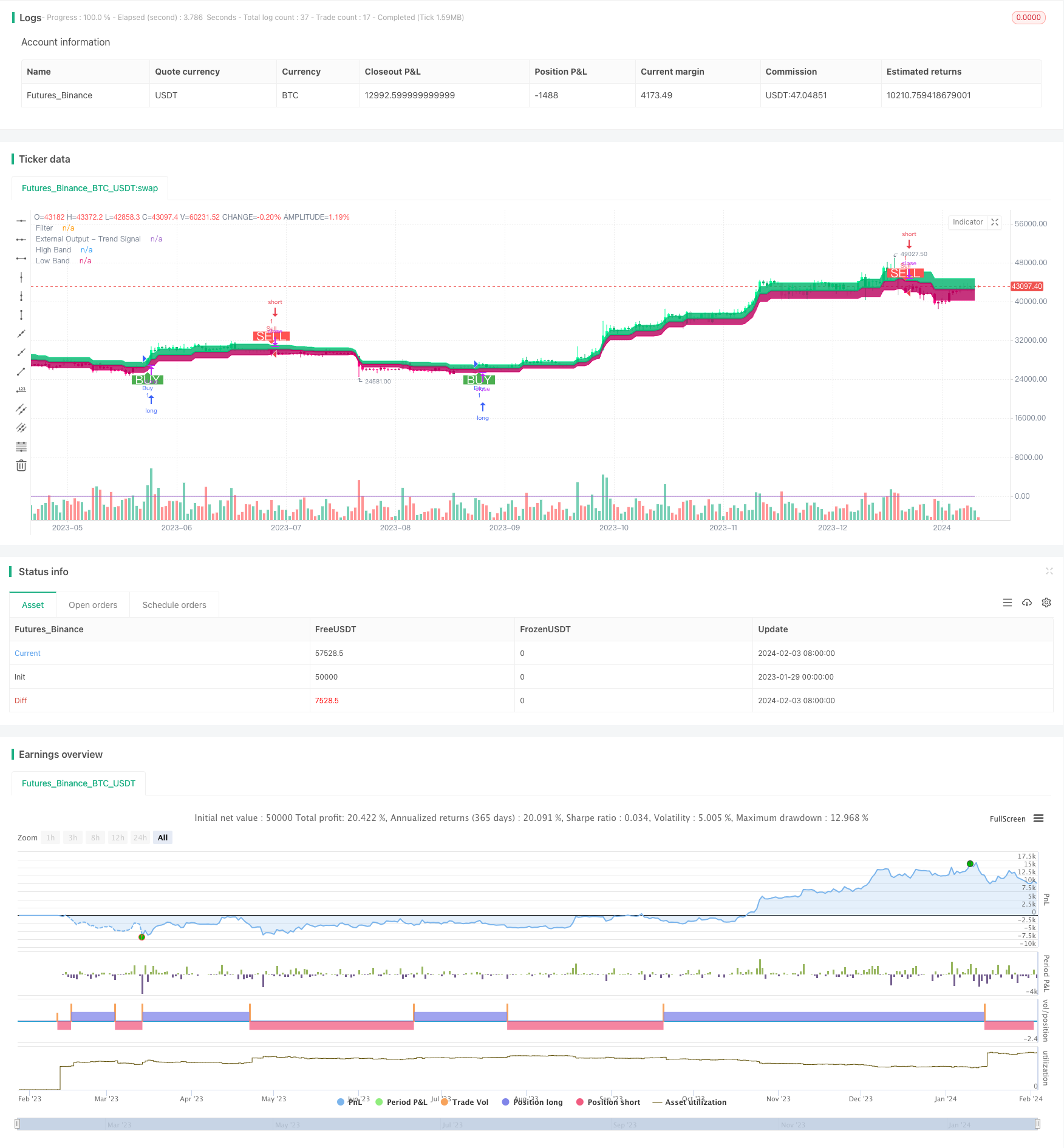
La Estrategia de seguimiento de tendencias de filtro de doble rango es una estrategia de negociación cuantitativa que utiliza el filtro de rango EMA dual para identificar la dirección de la tendencia y rastrear las tendencias.

Estrategia lógica

El núcleo de esta estrategia es el filtro de rango EMA dual. Calcula el rango ATR de las velas y lo suaviza, luego utiliza dos EMA para localizar la posición de las velas dentro del rango para determinar si actualmente está en una tendencia. Cuando el precio rompe el rango, señala un cambio en la tendencia.

Específicamente, la estrategia primero calcula el tamaño del rango ATR de las velas, y luego lo suaviza con dos EMA. El rango ATR representa el rango de fluctuación normal de las velas. Cuando el precio excede este rango, significa que se ha producido un cambio en la tendencia. La estrategia registra la dirección cuando el precio rompe el rango EMA. Cuando la dirección cambia, significa que se ha producido una inversión de tendencia, y es entonces cuando puede elegir entrar en el mercado.

Después de entrar en el mercado, la estrategia utiliza un stop loss flotante para bloquear las ganancias. Durante el período de retención, juzga constantemente si el candelabro ha caído fuera del rango. Si ocurre un retroceso, saldrá de la posición actual. Esto puede bloquear efectivamente las ganancias del comercio de tendencia.

Análisis de ventajas

La estrategia de seguimiento de tendencias de filtro de rango doble combina las ventajas del filtrado de promedios móviles y el cálculo de rango para determinar con precisión la dirección de la tendencia y evita entrar y salir con frecuencia del mercado en mercados de rango.

Utilice el principio ATR para juzgar el rango de fluctuación del candelabro, evita entrar en el mercado sin dirección durante el mercado de rango
El doble filtro EMA mejora la precisión del juicio y reduce las señales falsas
El stop loss flotante en tiempo real puede bloquear eficazmente las ganancias de tendencia
Lógica de estrategia simple y clara, fácil de entender y optimizar

Análisis de riesgos

Esta estrategia también presenta algunos riesgos, principalmente en los siguientes aspectos:

Las grandes lagunas pueden romper el rango de ATR, lo que resulta en una entrada prematura
En los mercados con tendencias fuertes, el stop loss puede activarse prematuramente
La configuración incorrecta de los parámetros también afecta el rendimiento de la estrategia

Para hacer frente a estos riesgos, se pueden utilizar métodos tales como optimizar los parámetros adecuadamente, prevenir falsas rupturas, juzgar la fuerza de la tendencia para resolverlos.

Sugerencias para optimizar

La estrategia de seguimiento de tendencias de filtros de doble alcance también tiene potencial para una mayor optimización, con las principales direcciones de optimización que incluyen:

Optimizar los parámetros ATR para suavizar el rango de fluctuación de las velas
Incorporar indicadores de volumen para evitar falsas rupturas
Evaluar la fuerza de la tendencia para distinguir entre las rupturas puntuales y las tendencias sostenibles
Optimizar el precio de stop loss para rastrear las tendencias largas y garantizar el beneficio

A través de estas optimizaciones, la estrategia puede lograr ganancias constantes en más entornos de mercado.

Resumen de las actividades

La estrategia de seguimiento de tendencias de filtro de doble rango integra las diversas ventajas del filtrado de promedios móviles y el juicio del rango ATR, y puede identificar efectivamente la dirección y el momento de entrada de tendencias sostenibles a medio y largo plazo. Solo entra en el mercado cuando cambian las tendencias y utiliza un stop loss flotante para bloquear las ganancias. Esta estrategia tiene una lógica simple y clara y es muy adecuada para el comercio de tendencias a medio y largo plazo. A través de la optimización continua de parámetros y reglas de juicio, esta estrategia puede lograr buenos rendimientos en varios mercados.

/*backtest
start: 2023-01-29 00:00:00
end: 2024-02-04 00:00:00
period: 1d
basePeriod: 1h
exchanges: [{"eid":"Futures_Binance","currency":"BTC_USDT"}]
*/

//@version=4
strategy("Range Filter [DW] & Labels", shorttitle="RF [DW] & Labels", overlay=true)

//Conditional Sampling EMA Function 
Cond_EMA(x, cond, n)=>
    var val     = array.new_float(0)
    var ema_val = array.new_float(1)
    if cond
        array.push(val, x)
        if array.size(val) > 1
            array.remove(val, 0)
        if na(array.get(ema_val, 0))
            array.fill(ema_val, array.get(val, 0))
        array.set(ema_val, 0, (array.get(val, 0) - array.get(ema_val, 0))*(2/(n + 1)) + array.get(ema_val, 0))
    EMA = array.get(ema_val, 0)
    EMA

//Conditional Sampling SMA Function
Cond_SMA(x, cond, n)=>
    var vals = array.new_float(0)
    if cond
        array.push(vals, x)
        if array.size(vals) > n
            array.remove(vals, 0)
    SMA = array.avg(vals)
    SMA

//Standard Deviation Function
Stdev(x, n)=>
    sqrt(Cond_SMA(pow(x, 2), 1, n) - pow(Cond_SMA(x, 1, n), 2))

//Range Size Function
rng_size(x, scale, qty, n)=> 
    ATR      = Cond_EMA(tr(true), 1, n)
    AC       = Cond_EMA(abs(x - x[1]), 1, n)
    SD       = Stdev(x, n)
    rng_size = scale=="Pips" ? qty*0.0001 : scale=="Points" ? qty*syminfo.pointvalue : scale=="% of Price" ? close*qty/100 : scale=="ATR" ? qty*ATR :
               scale=="Average Change" ? qty*AC : scale=="Standard Deviation" ? qty*SD : scale=="Ticks" ? qty*syminfo.mintick : qty   

//Two Type Range Filter Function
rng_filt(h, l, rng_, n, type, smooth, sn, av_rf, av_n)=>
    rng_smooth = Cond_EMA(rng_, 1, sn)
    r          = smooth ? rng_smooth : rng_
    var rfilt  = array.new_float(2, (h + l)/2)
    array.set(rfilt, 1, array.get(rfilt, 0))
    if type=="Type 1"
        if h - r > array.get(rfilt, 1)
            array.set(rfilt, 0, h - r)
        if l + r < array.get(rfilt, 1)
            array.set(rfilt, 0, l + r)
    if type=="Type 2"
        if h >= array.get(rfilt, 1) + r
            array.set(rfilt, 0, array.get(rfilt, 1) + floor(abs(h - array.get(rfilt, 1))/r)*r)
        if l <= array.get(rfilt, 1) - r
            array.set(rfilt, 0, array.get(rfilt, 1) - floor(abs(l - array.get(rfilt, 1))/r)*r)
    rng_filt1 = array.get(rfilt, 0)
    hi_band1  = rng_filt1 + r
    lo_band1  = rng_filt1 - r
    rng_filt2 = Cond_EMA(rng_filt1, rng_filt1 != rng_filt1[1], av_n)
    hi_band2  = Cond_EMA(hi_band1, rng_filt1 != rng_filt1[1], av_n)
    lo_band2  = Cond_EMA(lo_band1, rng_filt1 != rng_filt1[1], av_n)
    rng_filt  = av_rf ? rng_filt2 : rng_filt1
    hi_band   = av_rf ? hi_band2 : hi_band1
    lo_band   = av_rf ? lo_band2 : lo_band1
    [hi_band, lo_band, rng_filt]
 
//-----------------------------------------------------------------------------------------------------------------------------------------------------------------
//Inputs
//-----------------------------------------------------------------------------------------------------------------------------------------------------------------

//Filter Type
f_type = input(defval="Type 1", options=["Type 1", "Type 2"], title="Filter Type")

//Movement Source
mov_src = input(defval="Close", options=["Wicks", "Close"], title="Movement Source")

//Range Size Inputs
rng_qty   = input(defval=2.618, minval=0.0000001, title="Range Size")
rng_scale = input(defval="Average Change", options=["Points", "Pips", "Ticks", "% of Price", "ATR", "Average Change", "Standard Deviation", "Absolute"], title="Range Scale")

//Range Period
rng_per = input(defval=14, minval=1, title="Range Period (for ATR, Average Change, and Standard Deviation)")

//Range Smoothing Inputs
smooth_range = input(defval=true, title="Smooth Range")
smooth_per   = input(defval=27, minval=1, title="Smoothing Period")

//Filter Value Averaging Inputs
av_vals    = input(defval=true, title="Average Filter Changes")
av_samples = input(defval=2, minval=1, title="Number Of Changes To Average")

// New inputs for take profit and stop loss
take_profit_percent = input(defval=100.0, minval=0.1, maxval=1000.0, title="Take Profit Percentage", step=0.1)
stop_loss_percent = input(defval=100, minval=0.1, maxval=1000.0, title="Stop Loss Percentage", step=0.1)

//-----------------------------------------------------------------------------------------------------------------------------------------------------------------
//Definitions
//-----------------------------------------------------------------------------------------------------------------------------------------------------------------

//High And Low Values
h_val = mov_src=="Wicks" ? high : close
l_val = mov_src=="Wicks" ? low : close

//Range Filter Values
[h_band, l_band, filt] = rng_filt(h_val, l_val, rng_size((h_val + l_val)/2, rng_scale, rng_qty, rng_per), rng_per, f_type, smooth_range, smooth_per, av_vals, av_samples)

//Direction Conditions
var fdir = 0.0
fdir    := filt > filt[1] ? 1 : filt < filt[1] ? -1 : fdir
upward   = fdir==1 ? 1 : 0
downward = fdir==-1 ? 1 : 0

//Colors
filt_color = upward ? #05ff9b : downward ? #ff0583 : #cccccc
bar_color  = upward and (close > filt) ? (close > close[1] ? #05ff9b : #00b36b) :
             downward and (close < filt) ? (close < close[1] ? #ff0583 : #b8005d) : #cccccc

//-----------------------------------------------------------------------------------------------------------------------------------------------------------------
//Outputs
//-----------------------------------------------------------------------------------------------------------------------------------------------------------------

//Filter Plot
filt_plot = plot(filt, color=filt_color, transp=0, linewidth=3,  title="Filter")

//Band Plots
h_band_plot = plot(h_band, color=#05ff9b, transp=100, title="High Band")
l_band_plot = plot(l_band, color=#ff0583, transp=100, title="Low Band")

//Band Fills
fill(h_band_plot, filt_plot, color=#00b36b, transp=85, title="High Band Fill")
fill(l_band_plot, filt_plot, color=#b8005d, transp=85, title="Low Band Fill")

//Bar Color
barcolor(bar_color)

//External Trend Output
plot(fdir, transp=100, editable=false, display=display.none, title="External Output - Trend Signal")

// Trading Conditions Logic
longCond = close > filt and close > close[1] and upward > 0 or close > filt and close < close[1] and upward > 0 
shortCond = close < filt and close < close[1] and downward > 0 or close < filt and close > close[1] and downward > 0

CondIni = 0
CondIni := longCond ? 1 : shortCond ? -1 : CondIni[1]
longCondition = longCond and CondIni[1] == -1
shortCondition = shortCond and CondIni[1] == 1

// Strategy Entry and Exit
strategy.entry("Buy", strategy.long, when = longCondition)
strategy.entry("Sell", strategy.short, when = shortCondition)

// New: Close conditions based on percentage change
long_take_profit_condition = close > strategy.position_avg_price * (1 + take_profit_percent / 100)
short_take_profit_condition = close < strategy.position_avg_price * (1 - take_profit_percent / 100)

long_stop_loss_condition = close < strategy.position_avg_price * (1 - stop_loss_percent / 100)
short_stop_loss_condition = close > strategy.position_avg_price * (1 + stop_loss_percent / 100)

strategy.close("Buy", when = shortCondition or long_take_profit_condition or long_stop_loss_condition)
strategy.close("Sell", when = longCondition or short_take_profit_condition or short_stop_loss_condition)

// Plot Buy and Sell Labels
plotshape(longCondition, title = "Buy Signal", text ="BUY", textcolor = color.white, style=shape.labelup, size = size.normal, location=location.belowbar, color = color.green, transp = 0)
plotshape(shortCondition, title = "Sell Signal", text ="SELL", textcolor = color.white, style=shape.labeldown, size = size.normal, location=location.abovebar, color = color.red, transp = 0)

// Alerts
alertcondition(longCondition, title="Buy Alert", message = "BUY")
alertcondition(shortCondition, title="Sell Alert", message = "SELL")

Más.