Stratégie d'arbitrage statistique adaptatif de suivi du momentum


Date de création: 2023-12-11 16:41:27 Dernière modification: 2023-12-11 16:41:27
Copier: 0 Nombre de clics: 791
1
Suivre
1621
Abonnés

Stratégie d’arbitrage statistique adaptatif de suivi du momentum

Aperçu

La stratégie est basée sur la méthode de régression nucléaire de Nadaraya-Watson pour construire une zone de couverture dynamique de la volatilité, permettant un signal de transaction à bas prix et à haut prix en suivant l’intersection des prix avec la zone de couverture. La stratégie est basée sur l’analyse mathématique et peut s’adapter aux changements du marché.

Principe de stratégie

Le cœur de la stratégie est de calculer la courbe de couverture dynamique des prix. Tout d’abord, en fonction de la période de révision personnalisée, construire la courbe de régression nucléaire de Nadaraya-Watson pour les prix (… prix de clôture, prix le plus élevé, prix le plus bas) et obtenir une estimation de prix lissée. Ensuite, calculer l’indicateur ATR sur la base de la longueur ATR personnalisée, combinant les facteurs proches et éloignés, pour obtenir la portée de la bande de couverture supérieure et inférieure.

Avantages stratégiques

  1. Basé sur des modèles mathématiques, les paramètres sont contrôlables et il n’est pas facile de produire une optimisation excessive.
  2. Adapter à l’évolution du marché et saisir les opportunités de négociation grâce à la dynamique des prix et de la volatilité
  3. Utilisation de coordonnées logarithmiques pour une bonne gestion des variétés à différentes périodes de temps et à différentes amplitudes de fluctuation
  4. Sensibilité de la stratégie à des paramètres personnalisables

Risque stratégique

  1. Les modèles mathématiques sont théoriques, les disques peuvent être moins performants que prévu
  2. La sélection des paramètres clés nécessite de l’expérience, une mauvaise configuration peut affecter les gains
  3. Il y a un certain retard et des opportunités de transactions pourraient être manquées.
  4. Des signaux erronés dans un marché en pleine évolution

Il est essentiel d’éviter et de réduire ces risques en optimisant les paramètres, en effectuant un retour d’expérience, en connaissant les facteurs d’impact et en prenant des précautions concrètes.

Orientation de l’optimisation de la stratégie

  1. Optimiser les paramètres pour trouver la meilleure combinaison de paramètres
  2. Paramètres de sélection automatique utilisant l’apprentissage automatique
  3. Augmentation des conditions de filtrage et activation des stratégies dans des environnements de marché spécifiques
  4. Filtrage des signaux trompeurs en combinaison avec d’autres indicateurs
  5. Essayez différents modèles mathématiques

Résumer

La stratégie intègre l’analyse statistique et l’analyse des indicateurs techniques, permettant de suivre les prix et les fluctuations de manière dynamique. Elle permet d’ajuster les paramètres en fonction du marché et de ses propres conditions.
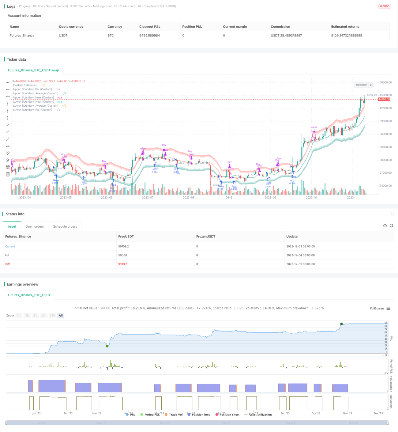
Code source de la stratégie
/*backtest
start: 2022-12-04 00:00:00
end: 2023-12-10 00:00:00
period: 1d
basePeriod: 1h
exchanges: [{"eid":"Futures_Binance","currency":"BTC_USDT"}]
*/

// © Julien_Eche
//@version=5

strategy("Nadaraya-Watson Envelope Strategy", overlay=true, pyramiding=1, default_qty_type=strategy.percent_of_equity, default_qty_value=20)

// Helper Functions
getEnvelopeBounds(_atr, _nearFactor, _farFactor, _envelope) => 
    _upperFar = _envelope + _farFactor*_atr
    _upperNear = _envelope + _nearFactor*_atr
    _lowerNear = _envelope - _nearFactor*_atr
    _lowerFar = _envelope - _farFactor*_atr
    _upperAvg = (_upperFar + _upperNear) / 2
    _lowerAvg = (_lowerFar + _lowerNear) / 2 
    [_upperNear, _upperFar, _upperAvg, _lowerNear, _lowerFar, _lowerAvg]

customATR(length, _high, _low, _close) =>
    trueRange = na(_high[1])? math.log(_high)-math.log(_low) : math.max(math.max(math.log(_high) - math.log(_low), math.abs(math.log(_high) - math.log(_close[1]))), math.abs(math.log(_low) - math.log(_close[1])))
    ta.rma(trueRange, length)

customKernel(x, h, alpha, x_0) =>
    sumWeights = 0.0
    sumXWeights = 0.0
    for i = 0 to h
        weight = math.pow(1 + (math.pow((x_0 - i), 2) / (2 * alpha * h * h)), -alpha)
        sumWeights := sumWeights + weight
        sumXWeights := sumXWeights + weight * x[i]
    sumXWeights / sumWeights

// Custom Settings
customLookbackWindow = input.int(8, 'Lookback Window (Custom)', group='Custom Settings')
customRelativeWeighting = input.float(8., 'Relative Weighting (Custom)', step=0.25, group='Custom Settings')
customStartRegressionBar = input.int(25, "Start Regression at Bar (Custom)", group='Custom Settings')

// Envelope Calculations
customEnvelopeClose = math.exp(customKernel(math.log(close), customLookbackWindow, customRelativeWeighting, customStartRegressionBar))
customEnvelopeHigh = math.exp(customKernel(math.log(high), customLookbackWindow, customRelativeWeighting, customStartRegressionBar))
customEnvelopeLow = math.exp(customKernel(math.log(low), customLookbackWindow, customRelativeWeighting, customStartRegressionBar))
customEnvelope = customEnvelopeClose
customATRLength = input.int(60, 'ATR Length (Custom)', minval=1, group='Custom Settings')
customATR = customATR(customATRLength, customEnvelopeHigh, customEnvelopeLow, customEnvelopeClose)
customNearATRFactor = input.float(1.5, 'Near ATR Factor (Custom)', minval=0.5, step=0.25, group='Custom Settings')
customFarATRFactor = input.float(2.0, 'Far ATR Factor (Custom)', minval=1.0, step=0.25, group='Custom Settings')
[customUpperNear, customUpperFar, customUpperAvg, customLowerNear, customLowerFar, customLowerAvg] = getEnvelopeBounds(customATR, customNearATRFactor, customFarATRFactor, math.log(customEnvelopeClose))

// Colors
customUpperBoundaryColorFar = color.new(color.red, 60)
customUpperBoundaryColorNear = color.new(color.red, 80)
customBullishEstimatorColor = color.new(color.teal, 50)
customBearishEstimatorColor = color.new(color.red, 50)
customLowerBoundaryColorNear = color.new(color.teal, 80)
customLowerBoundaryColorFar = color.new(color.teal, 60)

// Plots
customUpperBoundaryFar = plot(math.exp(customUpperFar), color=customUpperBoundaryColorFar, title='Upper Boundary: Far (Custom)')
customUpperBoundaryAvg = plot(math.exp(customUpperAvg), color=customUpperBoundaryColorNear, title='Upper Boundary: Average (Custom)')
customUpperBoundaryNear = plot(math.exp(customUpperNear), color=customUpperBoundaryColorNear, title='Upper Boundary: Near (Custom)') 
customEstimationPlot = plot(customEnvelopeClose, color=customEnvelope > customEnvelope[1] ? customBullishEstimatorColor : customBearishEstimatorColor, linewidth=2, title='Custom Estimation')
customLowerBoundaryNear = plot(math.exp(customLowerNear), color=customLowerBoundaryColorNear, title='Lower Boundary: Near (Custom)')
customLowerBoundaryAvg = plot(math.exp(customLowerAvg), color=customLowerBoundaryColorNear, title='Lower Boundary: Average (Custom)') 
customLowerBoundaryFar = plot(math.exp(customLowerFar), color=customLowerBoundaryColorFar, title='Lower Boundary: Far (Custom)')

// Fills
fill(customUpperBoundaryFar, customUpperBoundaryAvg, color=customUpperBoundaryColorFar, title='Upper Boundary: Farmost Region (Custom)')
fill(customUpperBoundaryNear, customUpperBoundaryAvg, color=customUpperBoundaryColorNear, title='Upper Boundary: Nearmost Region (Custom)')
fill(customLowerBoundaryNear, customLowerBoundaryAvg, color=customLowerBoundaryColorNear, title='Lower Boundary: Nearmost Region (Custom)')
fill(customLowerBoundaryFar, customLowerBoundaryAvg, color=customLowerBoundaryColorFar, title='Lower Boundary: Farmost Region (Custom)')


longCondition = ta.crossover(close, customEnvelopeLow)
if (longCondition)
    strategy.entry("Buy", strategy.long)

exitLongCondition = ta.crossover(customEnvelopeHigh, close)
if (exitLongCondition)
    strategy.close("Buy")