Stratégie de suivi des tendances des filtres à double portée

Auteur:ChaoZhang est là., Date: 2024-02-05 11h15 et 28 min
Les étiquettes:

Résumé

La stratégie de suivi de tendance du double filtrage de plage est une stratégie de trading quantitative qui utilise le double filtrage de plage EMA pour identifier la direction de la tendance et suivre les tendances.

La logique de la stratégie

Le noyau de cette stratégie est le double filtrage de la gamme EMA. Il calcule la gamme ATR des chandeliers et l'assouplit, puis utilise deux EMA pour localiser la position des chandeliers dans la gamme pour déterminer si elle est actuellement dans une tendance.

Plus précisément, la stratégie calcule d'abord la taille de la plage ATR des chandeliers, puis l'assouplit avec deux EMA. La plage ATR représente la plage de fluctuation normale des chandeliers. Lorsque le prix dépasse cette plage, cela signifie qu'un changement de tendance s'est produit. La stratégie enregistre la direction lorsque le prix franchit la plage EMA. Lorsque la direction change, cela signifie qu'un renversement de tendance s'est produit, et c'est à ce moment-là qu'elle peut choisir d'entrer sur le marché.

Après être entré sur le marché, la stratégie utilise un stop-loss flottant pour verrouiller les bénéfices. Pendant la période de détention, elle juge constamment si le chandelier est tombé hors de la plage. Si un repli se produit, elle sortira de la position actuelle. Cela peut effectivement verrouiller les bénéfices du trading de tendance.

Analyse des avantages

La stratégie de suivi des tendances du filtre à double plage combine les avantages du filtrage des moyennes mobiles et du calcul de la plage pour déterminer avec précision la direction de la tendance et éviter d'entrer et de sortir fréquemment du marché sur des marchés à plage.

Utilisez le principe ATR pour juger de la plage de fluctuation du chandelier, évite d'entrer sur le marché sans direction pendant la plage de marché
Le double filtre EMA améliore la précision du jugement et réduit les faux signaux
Le stop-loss flottant en temps réel peut effectivement bloquer les profits de tendance
Logie de stratégie simple et claire, facile à comprendre et à optimiser

Analyse des risques

Cette stratégie comporte également certains risques, principalement dans les aspects suivants:

Les grands trous peuvent briser la plage ATR, entraînant une entrée prématurée
Dans les marchés à forte tendance, le stop loss peut être déclenché prématurément
Les paramètres mal réglés affectent également les performances de la stratégie

Pour faire face à ces risques, des méthodes telles que l'optimisation appropriée des paramètres, la prévention de fausses ruptures, le jugement de la force de la tendance peuvent être utilisées pour les résoudre.

Suggestions d'optimisation

La stratégie de suivi des tendances des filtres à double portée a également un potentiel d'optimisation supplémentaire, les principales directions d'optimisation incluant:

Optimiser les paramètres de l'ATR afin d'assurer la fluctuation de la plage des chandeliers
Incorporer des indicateurs de volume pour éviter les fausses ruptures
Évaluer la force de la tendance pour distinguer les ruptures ponctuelles et les tendances durables
Optimiser le prix de stop loss pour suivre les tendances à long terme tout en assurant le profit

Grâce à ces optimisations, la stratégie peut réaliser des bénéfices stables dans un plus grand nombre d'environnements de marché.

Résumé

La stratégie de suivi des tendances du filtre à double plage intègre les différents avantages du filtrage des moyennes mobiles et du jugement de la plage ATR, et peut identifier efficacement la direction et le calendrier d'entrée des tendances durables à moyen et long terme. Elle n'entre sur le marché que lorsque les tendances changent et utilise un stop loss flottant pour verrouiller les bénéfices. Cette stratégie a une logique simple et claire et est très adaptée au trading de tendances à moyen et long terme. Grâce à l'optimisation continue des paramètres et des règles de jugement, cette stratégie peut obtenir de bons rendements sur divers marchés.

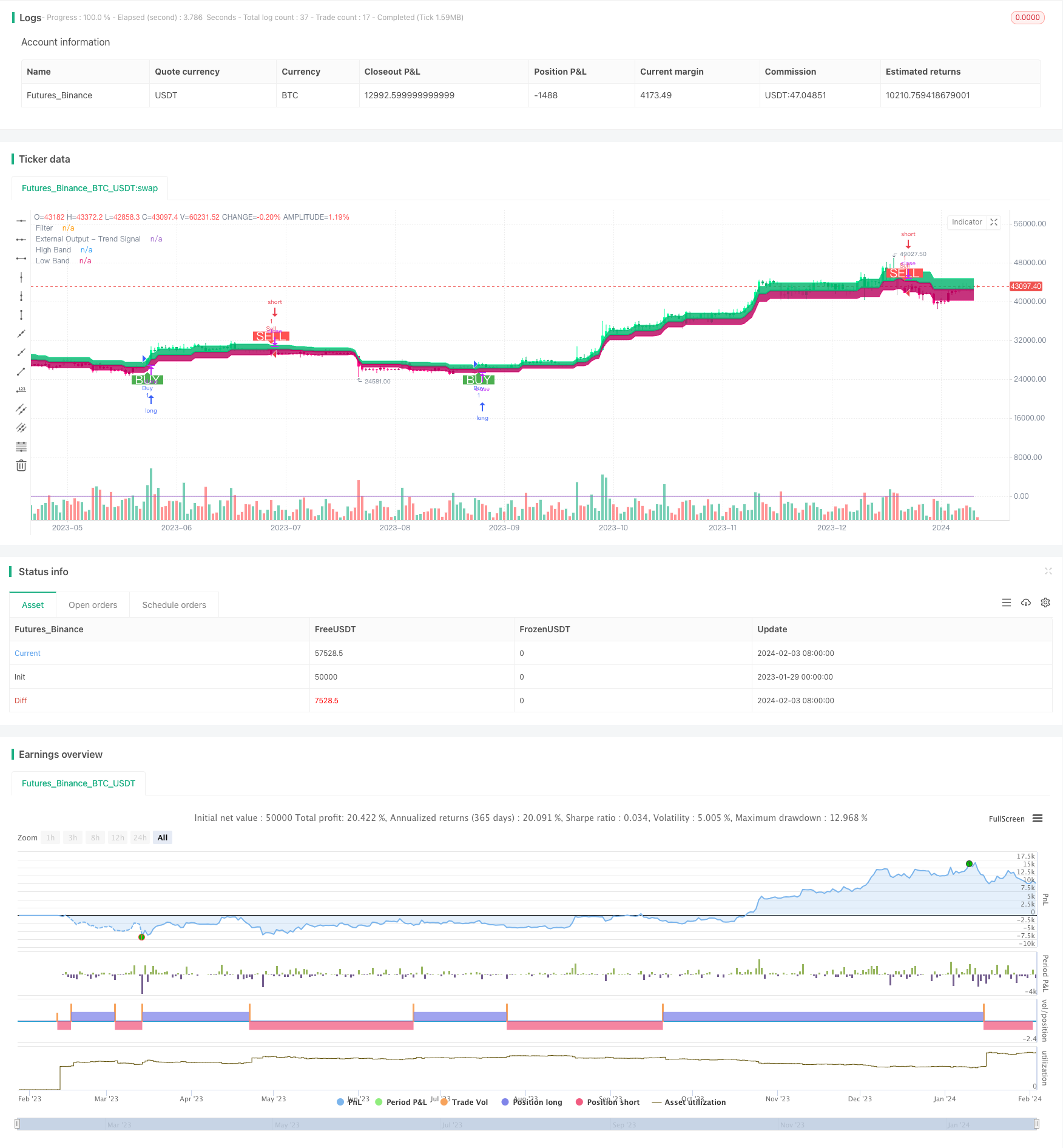
/*backtest
start: 2023-01-29 00:00:00
end: 2024-02-04 00:00:00
period: 1d
basePeriod: 1h
exchanges: [{"eid":"Futures_Binance","currency":"BTC_USDT"}]
*/

//@version=4
strategy("Range Filter [DW] & Labels", shorttitle="RF [DW] & Labels", overlay=true)

//Conditional Sampling EMA Function 
Cond_EMA(x, cond, n)=>
    var val     = array.new_float(0)
    var ema_val = array.new_float(1)
    if cond
        array.push(val, x)
        if array.size(val) > 1
            array.remove(val, 0)
        if na(array.get(ema_val, 0))
            array.fill(ema_val, array.get(val, 0))
        array.set(ema_val, 0, (array.get(val, 0) - array.get(ema_val, 0))*(2/(n + 1)) + array.get(ema_val, 0))
    EMA = array.get(ema_val, 0)
    EMA

//Conditional Sampling SMA Function
Cond_SMA(x, cond, n)=>
    var vals = array.new_float(0)
    if cond
        array.push(vals, x)
        if array.size(vals) > n
            array.remove(vals, 0)
    SMA = array.avg(vals)
    SMA

//Standard Deviation Function
Stdev(x, n)=>
    sqrt(Cond_SMA(pow(x, 2), 1, n) - pow(Cond_SMA(x, 1, n), 2))

//Range Size Function
rng_size(x, scale, qty, n)=> 
    ATR      = Cond_EMA(tr(true), 1, n)
    AC       = Cond_EMA(abs(x - x[1]), 1, n)
    SD       = Stdev(x, n)
    rng_size = scale=="Pips" ? qty*0.0001 : scale=="Points" ? qty*syminfo.pointvalue : scale=="% of Price" ? close*qty/100 : scale=="ATR" ? qty*ATR :
               scale=="Average Change" ? qty*AC : scale=="Standard Deviation" ? qty*SD : scale=="Ticks" ? qty*syminfo.mintick : qty   

//Two Type Range Filter Function
rng_filt(h, l, rng_, n, type, smooth, sn, av_rf, av_n)=>
    rng_smooth = Cond_EMA(rng_, 1, sn)
    r          = smooth ? rng_smooth : rng_
    var rfilt  = array.new_float(2, (h + l)/2)
    array.set(rfilt, 1, array.get(rfilt, 0))
    if type=="Type 1"
        if h - r > array.get(rfilt, 1)
            array.set(rfilt, 0, h - r)
        if l + r < array.get(rfilt, 1)
            array.set(rfilt, 0, l + r)
    if type=="Type 2"
        if h >= array.get(rfilt, 1) + r
            array.set(rfilt, 0, array.get(rfilt, 1) + floor(abs(h - array.get(rfilt, 1))/r)*r)
        if l <= array.get(rfilt, 1) - r
            array.set(rfilt, 0, array.get(rfilt, 1) - floor(abs(l - array.get(rfilt, 1))/r)*r)
    rng_filt1 = array.get(rfilt, 0)
    hi_band1  = rng_filt1 + r
    lo_band1  = rng_filt1 - r
    rng_filt2 = Cond_EMA(rng_filt1, rng_filt1 != rng_filt1[1], av_n)
    hi_band2  = Cond_EMA(hi_band1, rng_filt1 != rng_filt1[1], av_n)
    lo_band2  = Cond_EMA(lo_band1, rng_filt1 != rng_filt1[1], av_n)
    rng_filt  = av_rf ? rng_filt2 : rng_filt1
    hi_band   = av_rf ? hi_band2 : hi_band1
    lo_band   = av_rf ? lo_band2 : lo_band1
    [hi_band, lo_band, rng_filt]
 
//-----------------------------------------------------------------------------------------------------------------------------------------------------------------
//Inputs
//-----------------------------------------------------------------------------------------------------------------------------------------------------------------

//Filter Type
f_type = input(defval="Type 1", options=["Type 1", "Type 2"], title="Filter Type")

//Movement Source
mov_src = input(defval="Close", options=["Wicks", "Close"], title="Movement Source")

//Range Size Inputs
rng_qty   = input(defval=2.618, minval=0.0000001, title="Range Size")
rng_scale = input(defval="Average Change", options=["Points", "Pips", "Ticks", "% of Price", "ATR", "Average Change", "Standard Deviation", "Absolute"], title="Range Scale")

//Range Period
rng_per = input(defval=14, minval=1, title="Range Period (for ATR, Average Change, and Standard Deviation)")

//Range Smoothing Inputs
smooth_range = input(defval=true, title="Smooth Range")
smooth_per   = input(defval=27, minval=1, title="Smoothing Period")

//Filter Value Averaging Inputs
av_vals    = input(defval=true, title="Average Filter Changes")
av_samples = input(defval=2, minval=1, title="Number Of Changes To Average")

// New inputs for take profit and stop loss
take_profit_percent = input(defval=100.0, minval=0.1, maxval=1000.0, title="Take Profit Percentage", step=0.1)
stop_loss_percent = input(defval=100, minval=0.1, maxval=1000.0, title="Stop Loss Percentage", step=0.1)

//-----------------------------------------------------------------------------------------------------------------------------------------------------------------
//Definitions
//-----------------------------------------------------------------------------------------------------------------------------------------------------------------

//High And Low Values
h_val = mov_src=="Wicks" ? high : close
l_val = mov_src=="Wicks" ? low : close

//Range Filter Values
[h_band, l_band, filt] = rng_filt(h_val, l_val, rng_size((h_val + l_val)/2, rng_scale, rng_qty, rng_per), rng_per, f_type, smooth_range, smooth_per, av_vals, av_samples)

//Direction Conditions
var fdir = 0.0
fdir    := filt > filt[1] ? 1 : filt < filt[1] ? -1 : fdir
upward   = fdir==1 ? 1 : 0
downward = fdir==-1 ? 1 : 0

//Colors
filt_color = upward ? #05ff9b : downward ? #ff0583 : #cccccc
bar_color  = upward and (close > filt) ? (close > close[1] ? #05ff9b : #00b36b) :
             downward and (close < filt) ? (close < close[1] ? #ff0583 : #b8005d) : #cccccc

//-----------------------------------------------------------------------------------------------------------------------------------------------------------------
//Outputs
//-----------------------------------------------------------------------------------------------------------------------------------------------------------------

//Filter Plot
filt_plot = plot(filt, color=filt_color, transp=0, linewidth=3,  title="Filter")

//Band Plots
h_band_plot = plot(h_band, color=#05ff9b, transp=100, title="High Band")
l_band_plot = plot(l_band, color=#ff0583, transp=100, title="Low Band")

//Band Fills
fill(h_band_plot, filt_plot, color=#00b36b, transp=85, title="High Band Fill")
fill(l_band_plot, filt_plot, color=#b8005d, transp=85, title="Low Band Fill")

//Bar Color
barcolor(bar_color)

//External Trend Output
plot(fdir, transp=100, editable=false, display=display.none, title="External Output - Trend Signal")

// Trading Conditions Logic
longCond = close > filt and close > close[1] and upward > 0 or close > filt and close < close[1] and upward > 0 
shortCond = close < filt and close < close[1] and downward > 0 or close < filt and close > close[1] and downward > 0

CondIni = 0
CondIni := longCond ? 1 : shortCond ? -1 : CondIni[1]
longCondition = longCond and CondIni[1] == -1
shortCondition = shortCond and CondIni[1] == 1

// Strategy Entry and Exit
strategy.entry("Buy", strategy.long, when = longCondition)
strategy.entry("Sell", strategy.short, when = shortCondition)

// New: Close conditions based on percentage change
long_take_profit_condition = close > strategy.position_avg_price * (1 + take_profit_percent / 100)
short_take_profit_condition = close < strategy.position_avg_price * (1 - take_profit_percent / 100)

long_stop_loss_condition = close < strategy.position_avg_price * (1 - stop_loss_percent / 100)
short_stop_loss_condition = close > strategy.position_avg_price * (1 + stop_loss_percent / 100)

strategy.close("Buy", when = shortCondition or long_take_profit_condition or long_stop_loss_condition)
strategy.close("Sell", when = longCondition or short_take_profit_condition or short_stop_loss_condition)

// Plot Buy and Sell Labels
plotshape(longCondition, title = "Buy Signal", text ="BUY", textcolor = color.white, style=shape.labelup, size = size.normal, location=location.belowbar, color = color.green, transp = 0)
plotshape(shortCondition, title = "Sell Signal", text ="SELL", textcolor = color.white, style=shape.labeldown, size = size.normal, location=location.abovebar, color = color.red, transp = 0)

// Alerts
alertcondition(longCondition, title="Buy Alert", message = "BUY")
alertcondition(shortCondition, title="Sell Alert", message = "SELL")

Plus de

2019 FMZ - Tous les droits réservés