एल्स-स्मूथेड स्टोचैस्टिक आरएसआई रणनीति
अवलोकन
इस रणनीति का मुख्य विचार यह है कि एल्स सुपर स्मूथर फिल्टर का उपयोग करके स्टोकेस्टिक आरएसआई संकेतक को संसाधित किया जाए, जिससे कई झूठे संकेतों को फ़िल्टर किया जा सके और अधिक विश्वसनीय ट्रेडिंग सिग्नल प्राप्त किए जा सकें। मूल सिद्धांत यह है कि पहले यादृच्छिक मजबूत-कमज़ोर सूचकांक की गणना की जाए, फिर एल्स सुपर स्मूथर फिल्टर का उपयोग करके इसे संसाधित किया जाए, और अंत में अपने स्वयं के चलती औसत के साथ क्रॉस करें।
रणनीति सिद्धांत
इस रणनीति में पहले RSI को लॉग क्लोजर प्राइस पर गणना की जाती है और फिर RSI के आधार पर स्टोकेस्टिक को गणना की जाती है, जो कि एक अपेक्षाकृत कमजोर सूचकांक है। झूठे संकेतों को फ़िल्टर करने के लिए, स्टोकेस्टिक आरएसआई को एल्स सुपरप्लेट फ़िल्टर का उपयोग करके संसाधित किया जाता है, और अंत में स्टोकेस्टिक आरएसआई लाइन को अपनी खुद की चलती औसत के साथ गोल्ड क्रॉस-डायड किया जाता है, और क्रॉस को खाली कर दिया जाता है। इसलिए इस रणनीति के लिए महत्वपूर्ण बिंदु हैंः 1) स्टोकेस्टिक आरएसआई को गणना करें; 2) एल्स सुपरप्लेट फ़िल्टर का उपयोग करें; 3) एक ट्रेडिंग सिग्नल बनाने के लिए चलती औसत के साथ।
श्रेष्ठता विश्लेषण
इस रणनीति का सबसे बड़ा लाभ यह है कि एल्स सुपर स्मूथ फिल्टर का उपयोग किया जाता है, जो कई झूठे संकेतों को प्रभावी ढंग से फ़िल्टर करता है, जिससे ट्रेडिंग सिग्नल अधिक विश्वसनीय होते हैं। इसके अलावा, स्टोकेस्टिक आरएसआई संकेतक में स्वयं बहुत अच्छी ब्रेकआउट और ट्रेंड ट्रैकिंग क्षमता होती है। इसलिए यह रणनीति ट्रेंड को सही ढंग से पहचान सकती है, सही समय पर पोजीशन बना सकती है, सही समय पर पोजीशन को कम कर सकती है।
जोखिम विश्लेषण
इस रणनीति का मुख्य जोखिम यह है कि जब बाजार में भारी उतार-चढ़ाव होता है, तो यह गलत संकेतों के लिए अतिसंवेदनशील होता है। स्टोकेस्टिक आरएसआई संकेतक कई झूठे उछाल और गिरावट के संकेतों का उत्पादन करता है जब कीमतें एक संकीर्ण सीमा में भारी उतार-चढ़ाव करती हैं, और इस समय एल्स सुपर स्मूद फिल्टर की प्रभावशीलता भी छूट जाती है। इसके अलावा, कुछ चरम स्थितियों में, संकेतक की पिछड़ापन कुछ जोखिम भी ले सकती है।
इन जोखिमों को कम करने के लिए, स्टोकेस्टिक सूचक चक्र को बड़ा करने, चिकनाई को कम करने आदि जैसे मापदंडों को उचित रूप से समायोजित किया जा सकता है, जिससे झूठे संकेतों को और अधिक फ़िल्टर किया जा सके। इसके अलावा, अन्य संकेतकों या रूपों के साथ संयोजन पर विचार किया जा सकता है, जिससे कई फ़िल्टरिंग स्थितियां बनें और गलत संकेतों के जोखिम से बचा जा सके।
अनुकूलन दिशा
इस रणनीति को निम्नलिखित क्षेत्रों में अनुकूलित किया जा सकता हैः
ऑप्टिमाइज़ेशन पैरामीटर सेटिंग्स. स्टोचैस्टिक आरएसआई सूचक की लंबाई, चिकनाई स्थिरांक और अन्य जैसे पैरामीटरों का सावधानीपूर्वक परीक्षण किया जा सकता है ताकि सर्वोत्तम पैरामीटर संयोजन का पता लगाया जा सके।
बढ़ी हुई हानि तंत्र. लाभ को लॉक करने और निकासी को कम करने के लिए एक चलती रोक या एक लटकती रोक को सेट किया जा सकता है.
अन्य सूचकांकों या आकृति के साथ संयोजन. अस्थिरता सूचकांक, चलती औसत आदि के साथ संयोजन पर विचार किया जा सकता है, जिससे कई फ़िल्टरिंग स्थितियां बनती हैं और जोखिम को और कम किया जा सकता है।
बड़े चक्र विश्लेषण के परिणामों के आधार पर स्थिति को समायोजित करें। उच्च समय अवधि के रुझान विश्लेषण के परिणामों के आधार पर, गतिशील रूप से प्रत्येक व्यापार के लिए स्थिति के आकार को समायोजित करें।
संक्षेप
यह रणनीति पहले स्टोकेस्टिक आरएसआई संकेतक की गणना करती है, फिर इसे एल्स सुपर स्मूथ फिल्टर का उपयोग करके संसाधित करती है, और अंत में अपनी खुद की चलती औसत के साथ एक ट्रेडिंग सिग्नल बनाती है, जिससे रुझान का सही निर्णय किया जा सके। रणनीति का लाभ यह है कि संकेतक और फिल्टर के संयोजन का उपयोग किया जाता है, जिससे झूठे संकेतों को प्रभावी ढंग से फ़िल्टर किया जा सकता है और उच्च संभावना वाले व्यापार के अवसर प्राप्त किए जा सकते हैं। जोखिम मुख्य रूप से गलत पैरामीटर सेटिंग और स्टॉप लॉस तंत्र की कमी से आता है। पैरामीटर अनुकूलन, स्टॉप लॉस जोड़ने और संयोजन अनुकूलन जैसे तरीकों से रणनीति की स्थिरता और लाभप्रदता के स्तर को और बढ़ाया जा सकता है।
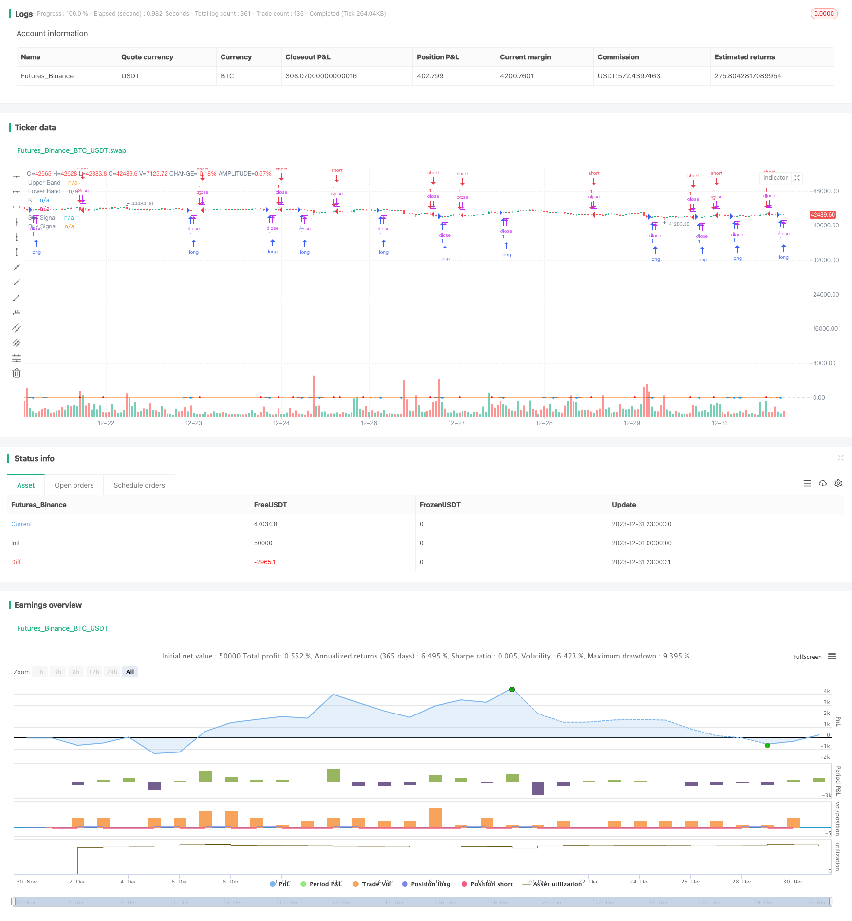
/*backtest
start: 2023-12-01 00:00:00
end: 2023-12-31 23:59:59
period: 1h
basePeriod: 15m
exchanges: [{"eid":"Futures_Binance","currency":"BTC_USDT"}]
*/

//@version=3
strategy("ES Stoch RSI Strategy [krypt]", overlay=true, calc_on_order_fills=true, calc_on_every_tick=true, initial_capital=10000, currency='USD')

//Backtest Range
FromMonth = input(defval = 06, title = "From Month", minval = 1)
FromDay   = input(defval = 1, title = "From Day", minval = 1)
FromYear  = input(defval = 2018, title = "From Year", minval = 2014)
ToMonth   = input(defval = 7, title = "To Month", minval = 1)
ToDay     = input(defval = 30, title = "To Day", minval = 1)
ToYear    = input(defval = 2018, title = "To Year", minval = 2014)

PI = 3.14159265359

drop1st(src) =>
    x = na
    x := na(src[1]) ? na : src

xlowest(src, len) =>
    x = src
    for i = 1 to len - 1
        v = src[i]
        if (na(v))
            break
        x := min(x, v)
    x

xhighest(src, len) =>
    x = src
    for i = 1 to len - 1
        v = src[i]
        if (na(v))
            break
        x := max(x, v)
    x

xstoch(c, h, l, len) =>
    xlow = xlowest(l, len)
    xhigh = xhighest(h, len)
    100 * (c - xlow) / (xhigh - xlow)

Stochastic(c, h, l, length) =>
    rawsig = xstoch(c, h, l, length)
    min(max(rawsig, 0.0), 100.0)

xrma(src, len) =>
    sum = na
    sum := (src + (len - 1) * nz(sum[1], src)) / len

xrsi(src, len) =>
    msig = nz(change(src, 1), 0.0)
    up = xrma(max(msig, 0.0), len)
    dn = xrma(max(-msig, 0.0), len)
    rs = up / dn
    100.0 - 100.0 / (1.0 + rs)

EhlersSuperSmoother(src, lower) =>
	a1 = exp(-PI * sqrt(2) / lower)
	coeff2 = 2 * a1 * cos(sqrt(2) * PI / lower)
	coeff3 = -pow(a1, 2)
	coeff1 = (1 - coeff2 - coeff3) / 2
	filt = na
	filt := nz(coeff1 * (src + nz(src[1], src)) + coeff2 * filt[1] + coeff3 * filt[2], src)

smoothK = input(7, minval=1, title="K")
smoothD = input(2, minval=1, title="D")
lengthRSI = input(10, minval=1, title="RSI Length")
lengthStoch = input(3, minval=1, title="Stochastic Length")
showsignals = input(true, title="Buy/Sell Signals")
src = input(close,  title="Source")

ob = 80
os = 20
midpoint = 50

price = log(drop1st(src))
rsi1 = xrsi(price, lengthRSI)
rawsig = Stochastic(rsi1, rsi1, rsi1, lengthStoch)
sig = EhlersSuperSmoother(rawsig, smoothK)
ma = sma(sig, smoothD)

plot(sig, color=#0094ff, title="K", transp=0)
plot(ma, color=#ff6a00, title="D", transp=0)
lineOB = hline(ob, title="Upper Band", color=#c0c0c0)
lineOS = hline(os, title="Lower Band", color=#c0c0c0)
fill(lineOB, lineOS, color=purple, title="Background")

// Buy/Sell Signals

// use curvature information to filter out some false positives
mm1 = change(change(ma, 1), 1)
mm2 = change(change(ma, 2), 2)
ms1 = change(change(sig, 1), 1)
ms2 = change(change(sig, 2), 2)

sellsignals = showsignals and (mm1 + ms1 < 0 and mm2 + ms2 < 0) and crossunder(sig, ma) and sig[1] > ob
buysignals = showsignals and (mm1 + ms1 > 0 and mm2 + ms2 > 0) and crossover(sig, ma) and sig[1] < os

ploff = 4
plot(buysignals ? sig[1] - ploff : na, style=circles, color=#008fff, linewidth=3, title="Buy Signal", transp=0)
plot(sellsignals ? sig[1] + ploff : na, style=circles, color=#ff0000, linewidth=3, title="Sell Signal", transp=0)

longCondition = buysignals
if (longCondition)
    strategy.entry("L", strategy.long, comment="Long", when=(buysignals))

shortCondition = sellsignals
if (shortCondition)
    strategy.entry("S", strategy.short, comment="Short", when=(sellsignals))