モメンタム追従型適応統計的裁定戦略

1
Follow
1779
Followers
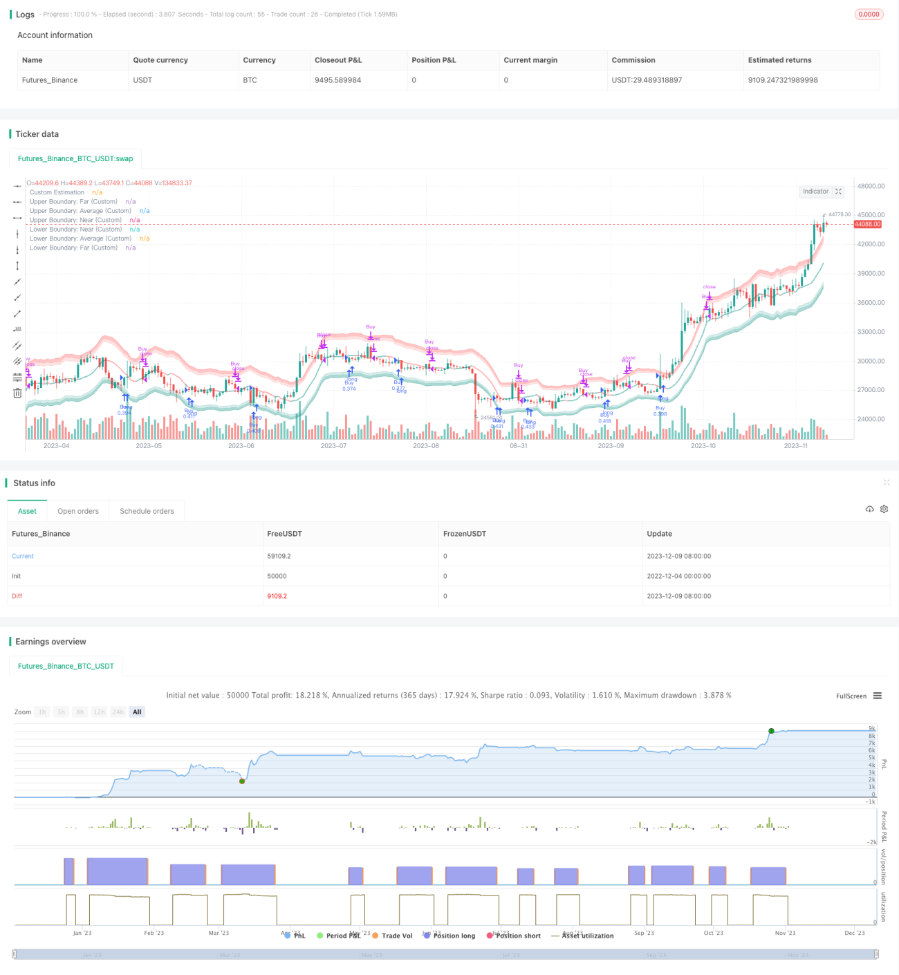
概要
この戦略は,Nadaraya-Watson核帰帰法に基づいて,動的波動率の包囲帯を構成し,価格と包囲帯の交差状況を追跡することによって,低価格で高価格で売る取引信号を実現する.この戦略は,数学分析の基礎を持ち,市場変化に自律的に適応する.
戦略原則
戦略の核心は,価格の動的包囲帯を計算することです. まず,カスタマイズされた回顧期に基づいて価格 ((閉店価格,最高価格,最低価格) のナダラヤ-ワトソン核回帰曲線を構成し,平らな価格見積もりを得ます. その後,カスタマイズされたATR長さのベースでATR指標を計算し,近端因子と遠端因子を組み合わせて,上下包囲帯の範囲を得ます.
戦略的優位性
- 数学モデルに基づく,パラメータは制御可能で,過剰最適化には容易ではない.
- 市場の変化に適応し,価格と変動のダイナミックな関係を利用して取引の機会を捉える
- 対数座標を使用し,異なる時間周期と波動幅の品種をうまく処理できます
- カスタマイズ可能なパラメータの調整策の感度
戦略リスク
- 数学モデル理論化,リッドディスクのパフォーマンスが予想より低い
- 重要なパラメータの選択は経験が必要で,不適切な設定は収益に影響を及ぼす可能性があります.
- 取引の機会を逃したかもしれない.
- 市場が大きく揺れ動いた時,誤ったシグナルが出る可能性が高い.
これらのリスクは,主にパラメータの最適化,反省,影響要因の理解,慎重な実盤によって回避および軽減されます.
戦略最適化の方向性
- パラメータをさらに最適化して,最適なパラメータの組み合わせを見つけます.
- 機械学習による自動選択パラメータ
- フィルタリング条件を追加し,特定の市場環境で戦略を活性化します.
- 他の指標と組み合わせたフィルタリング
- 異なる数学モデルのアルゴリズムを試す
要約する
この戦略は,統計分析と技術指標分析を統合し,価格と変動率を動的に追跡することによって,低価格と高価格の取引シグナルを実現する.市場と自身の状況に応じてパラメータを調整することができる.全体的に,戦略の理論的基盤は堅牢であり,実際のパフォーマンスはさらに検証される必要がある.慎重に観察し,慎重に実態を観察する必要があります.
Source
Pine
/*backtest
start: 2022-12-04 00:00:00
end: 2023-12-10 00:00:00
period: 1d
basePeriod: 1h
exchanges: [{"eid":"Futures_Binance","currency":"BTC_USDT"}]
*/

// © Julien_Eche
//@version=5

strategy("Nadaraya-Watson Envelope Strategy", overlay=true, pyramiding=1, default_qty_type=strategy.percent_of_equity, default_qty_value=20)Strategy parameters
Related strategies
Comment
All comments (0)
No data
- 1