動的移動平均クロスオーバー戦略

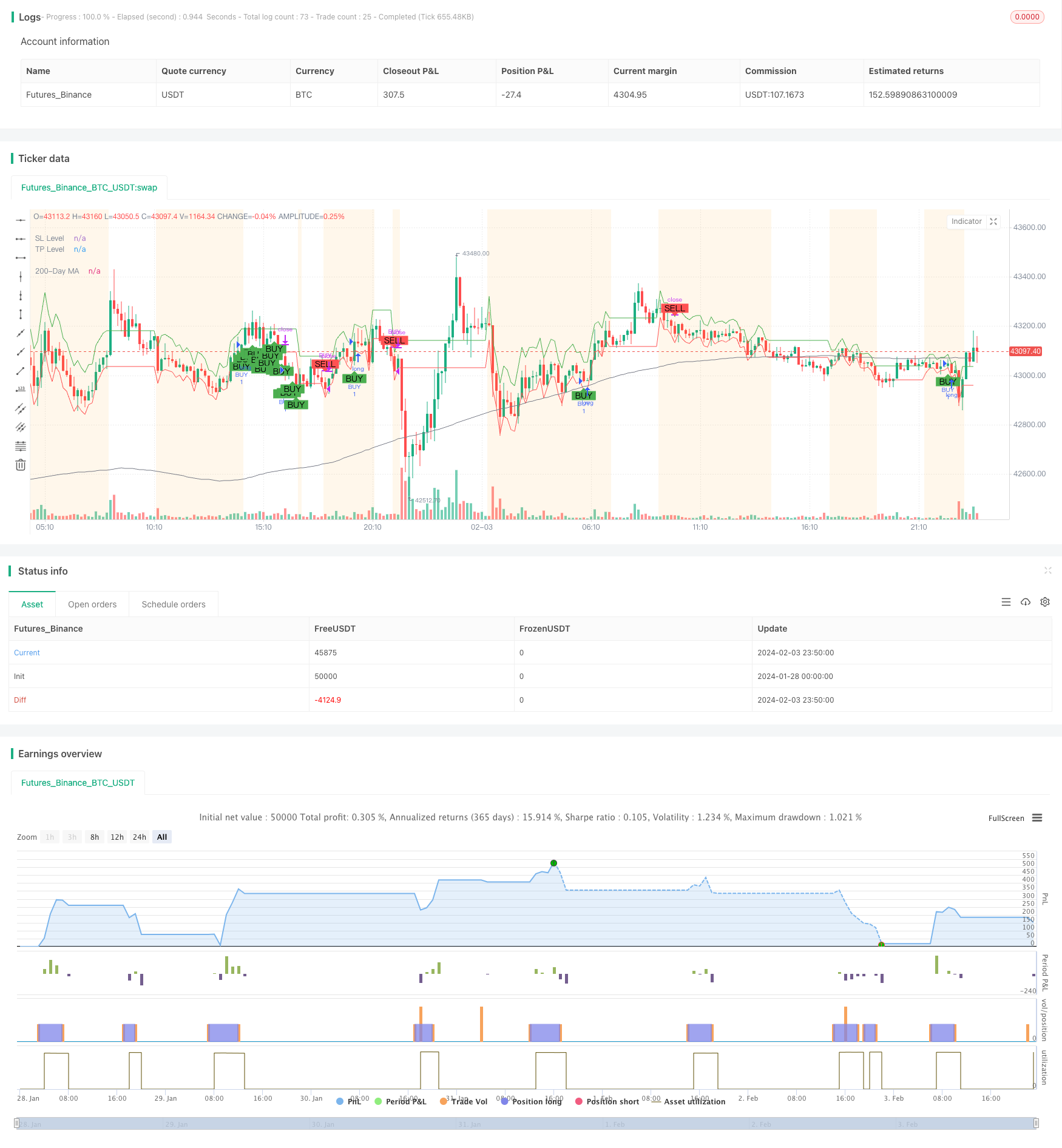
/*backtest
start: 2024-01-28 00:00:00
end: 2024-02-04 00:00:00
period: 10m
basePeriod: 1m
exchanges: [{"eid":"Futures_Binance","currency":"BTC_USDT"}]
*/

//@version=5
strategy("Improved Custom Strategy", shorttitle="ICS", overlay=true)

// Volatility
volatility = ta.atr(14)
avg_volatility_sma = ta.sma(volatility, 100)
avg_volatility = na(avg_volatility_sma) ? 0 : avg_volatility_sma

// Market Phase detection
long_term_ma = ta.sma(close, 200)
distance_from_long_term_ma = close - long_term_ma
var bool isTrending = math.abs(distance_from_long_term_ma) > 1.5 * avg_volatility and not na(distance_from_long_term_ma)
var bool isVolatile = volatility > 1.5 * avg_volatility

// EMA/MA Crossover
fast_length = 10
slow_length = 30
fast_ma = ta.ema(close, fast_length)
slow_ma = ta.sma(close, slow_length)
crossover_signal = ta.crossover(fast_ma, slow_ma)

// MACD
[macdLine, signalLine, macdHistogram] = ta.macd(close, 12, 26, 9)
macd_signal = crossover_signal or (macdHistogram > 0)

// Bollinger Bands
source = close
basis = ta.sma(source, 20)
upper = basis + 2 * ta.stdev(source, 20)
lower = basis - 2 * ta.stdev(source, 20)
isConsolidating = (upper - lower) < ta.sma(upper - lower, 20)

// StockRSI
length = 14
K = 100 * (close - ta.lowest(close, length)) / (ta.highest(close, length) - ta.lowest(close, length))
D = ta.sma(K, 3)
overbought = 75
oversold = 25

var float potential_SL = na
var float potential_TP = na
var bool buy_condition = na
var bool sell_condition = na

// Buy and Sell Control Variables
var bool hasBought = false
var bool hasSold = true

// Previous values tracking
prev_macdHistogram = macdHistogram[1]
prev_close = close[1]

// Modify sell_condition with the new criteria
if isVolatile
    buy_condition := not hasBought and crossover_signal or macd_signal and (close > lower) and (close < upper)
    sell_condition := hasBought and (macdHistogram < 0 and prev_macdHistogram < 0) and (close < prev_close and prev_close < close[2])
    potential_SL := close - 0.5 * volatility
    potential_TP := close + volatility

if isTrending
    buy_condition := not hasBought and crossover_signal or macd_signal
    sell_condition := hasBought and (macdHistogram < 0 and prev_macdHistogram < 0) and (close < prev_close and prev_close < close[2])
    potential_SL := close - volatility
    potential_TP := close + 2 * volatility

if isConsolidating
    buy_condition := not hasBought and crossover_signal and (close > lower)
    sell_condition := hasBought and (close < upper) and (macdHistogram < 0 and prev_macdHistogram < 0) and (close < prev_close and prev_close < close[2])
    potential_SL := close - 0.5 * volatility
    potential_TP := close + volatility

// Update the hasBought and hasSold flags
if buy_condition
    hasBought := true
    hasSold := false

if sell_condition
    hasBought := false
    hasSold := true

// Strategy Entry and Exit
if buy_condition
    strategy.entry("BUY", strategy.long, stop=potential_SL, limit=potential_TP)
    strategy.exit("SELL_TS", from_entry="BUY", trail_price=close, trail_offset=close * 0.05)

if sell_condition
    strategy.close("BUY")
    
// Visualization
plotshape(series=buy_condition, style=shape.labelup, location=location.belowbar, color=color.green, text="BUY", size=size.small)
plotshape(series=sell_condition, style=shape.labeldown, location=location.abovebar, color=color.red, text="SELL", size=size.small)

plot(long_term_ma, color=color.gray, title="200-Day MA", linewidth=1)
plot(potential_SL, title="SL Level", color=color.red, linewidth=1, style=plot.style_linebr)
plot(potential_TP, title="TP Level", color=color.green, linewidth=1, style=plot.style_linebr)

bgcolor(isVolatile ? color.new(color.purple, 90) : isTrending ? color.new(color.blue, 90) : isConsolidating ? color.new(color.orange, 90) : na)