개요
동적 이동 평균 교차 조합 전략 (Dynamic Moving Average Crossover Combo Strategy) 은 여러 가지 기술 지표와 시장 단계 검사를 통합한 복합 거래 전략이다. 그것은 동적으로 시장의 변동성을 계산하고, 가격과 장기 이동 평균의 거리 및 변동성에 따라 시장의 세 단계: 흔들림, 추세 및 정리한다. 전략은 시장의 다른 단계에서 다른 출구 규칙을 채택하며, 동시에 EMA/SMA 교차, MACD 및 볼링거래 밴드와 같은 여러 지표가 결합되어 구매 및 판매 신호를 발송한다.
전략 원칙
시장의 변동성을 계산하는 방법
ATR (Average True Rate of Volatility) 지표를 사용하여 최근 14 일 동안의 시장의 일일 변동성을 계산하십시오. 100 일 간 간단한 이동 평균 필터링을 사용하여 평균 변동성을 얻으십시오.
시장 단계 판단
가격의 200일 간소 이동 평균의 거리를 계산한다. 만약 거리가 평균 변동성의 1.5배를 초과하고 방향이 명확하다면, 추세상태로 판단한다. 만약 현재 변동성이 평균 변동성의 1.5배를 초과하면, 충격상태로 판단한다.
EMA/SMA 교차
빠른 EMA 주기는 10일이고, 느린 SMA 주기는 30일이다. 빠른 EMA 상에서 느린 SMA를 통과하면 구매 신호가 발생한다.
MACD
12, 26, 9의 매크드 변수를 계산한다. 매크드 기둥이 양이 되면 구매 신호가 발생한다.
Bollinger Bands
20일간의 표준차이를 계산하는 채널。 채널의 폭이 자신의 20일 SMA보다 작으면 정리 기간으로 판단한다。
참가 규칙
격동기: 빠른 속도로 선이 교차하거나 MACD 기둥이 교정되고, 그리고 마감 가격이 볼린저 밴드 안에 있다면, 입장은 더 많이 한다.
트렌드 기간: 빠른 느린 라인 크로스 또는 MACD 기둥 정규 입장이 더 많이 진행된다.
정리 기간: 빠른 속도로 선을 교차하고, 마감 가격이 Lower Band보다 높으면 입장이 더 많이 된다.
출전 규칙
다음 조건이 충족되면 평점으로 출장한다: MACD 연속 두 개의 K 선이 마이너스이며, 종결 가격은 연속 두 일 동안 하락했다.
위기상황: 주식 RSI가 초고가역에 진입했을 때 출전한다.
정렬 기간: 또한 가격이 Upper Band보다 낮을 때 출전한다.
우위 분석
이 전략은 시장 상황에 대한 판단과 함께 다음과 같은 장점을 갖는다.
체계화하고 주관적인 개입을 줄여라.
시장 환경 조정 전략의 매개 변수와 결합하여 더 잘 적응할 수 있습니다.
여러 지표의 조합으로 신호의 확실성을 높여줍니다.
Bollinger Bands는 자동으로 손실을 줄이고 위험을 줄입니다.
모든 조건을 판단하고, 가짜 신호를 필터링한다.
동적 스톱로스 스톱, 트렌드 추적 수익
위험 분석
주요 위험은 다음과 같습니다.
잘못된 매개 변수 설정으로 인해 정책이 실패할 수 있습니다. 매개 변수 조합을 최적화하는 것이 좋습니다.
급격한 사건으로 인해 모델이 작동하지 않습니다. 전략 논리를 업데이트하는 것이 좋습니다.
거래비용을 압축하여 수익을 얻을 수 있는 공간. 낮은 수수료의 증권사를 선택하는 것이 좋습니다.
다중 지표 조합은 전략의 복잡성을 증가시킵니다. 핵심 지표를 선택하는 것이 좋습니다.
최적화 방향
다음의 몇 가지 측면에서 더 최적화할 수 있습니다.
시장 환경 판단 기준을 최적화하고 정확도를 향상시킵니다.
기계 학습 모듈을 추가하여 파라미터 적응을 구현한다.
텍스트 처리와 결합하여 중대한 사건의 위험을 판단한다.
다중 시장 재검토, 최적의 조합을 찾는 것.
트레일링 스톱을 추가하는 전략.
요약하다
동적 이동 평균 십자조합 전략은 다중 지표 지능형 거래 전략이다. 그것은 시장 환경 조정 파라미터를 결합하여 조건 판단 방식의 체계화된 거래를 구현한다. 강한 적응성과 확실성을 가지고 있다. 그러나 파라미터 설정과 새로운 모듈은 전략의 복잡성을 증가시키지 않도록 주의해야 한다. 전체적으로 볼 때, 이것은 강력한 실행성 있는 정량화 전략이다.
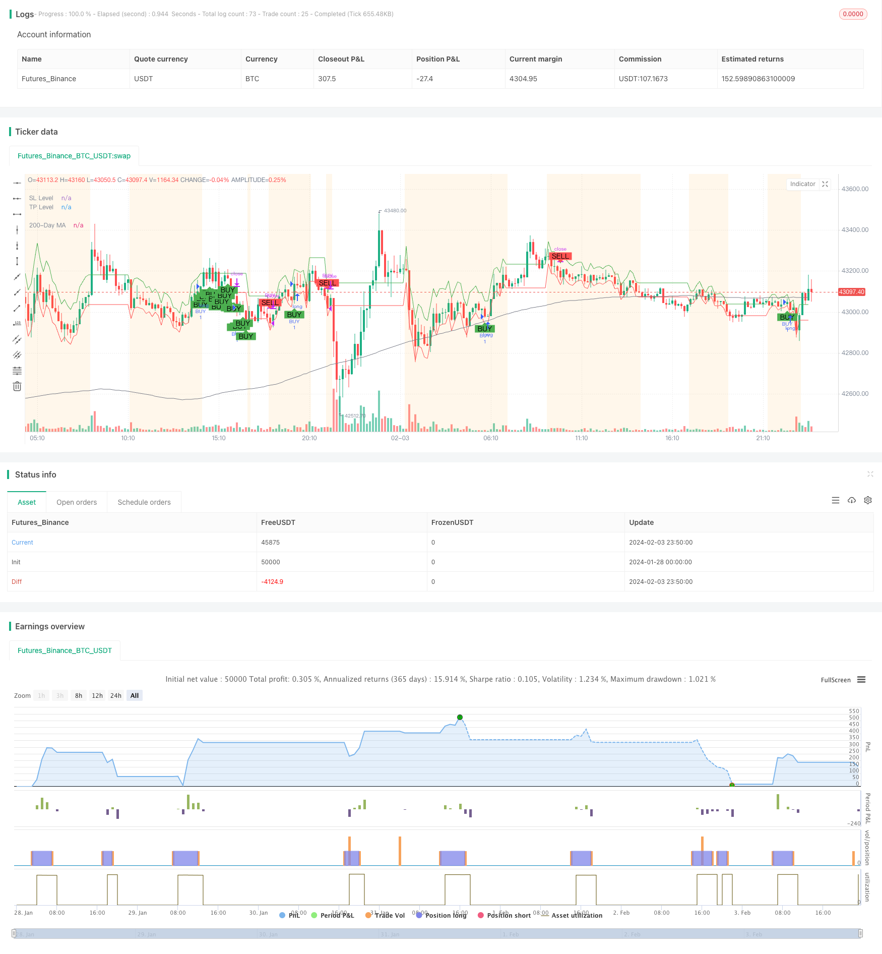
/*backtest
start: 2024-01-28 00:00:00
end: 2024-02-04 00:00:00
period: 10m
basePeriod: 1m
exchanges: [{"eid":"Futures_Binance","currency":"BTC_USDT"}]
*/

//@version=5
strategy("Improved Custom Strategy", shorttitle="ICS", overlay=true)

// Volatility
volatility = ta.atr(14)
avg_volatility_sma = ta.sma(volatility, 100)
avg_volatility = na(avg_volatility_sma) ? 0 : avg_volatility_sma

// Market Phase detection
long_term_ma = ta.sma(close, 200)
distance_from_long_term_ma = close - long_term_ma
var bool isTrending = math.abs(distance_from_long_term_ma) > 1.5 * avg_volatility and not na(distance_from_long_term_ma)
var bool isVolatile = volatility > 1.5 * avg_volatility

// EMA/MA Crossover
fast_length = 10
slow_length = 30
fast_ma = ta.ema(close, fast_length)
slow_ma = ta.sma(close, slow_length)
crossover_signal = ta.crossover(fast_ma, slow_ma)

// MACD
[macdLine, signalLine, macdHistogram] = ta.macd(close, 12, 26, 9)
macd_signal = crossover_signal or (macdHistogram > 0)

// Bollinger Bands
source = close
basis = ta.sma(source, 20)
upper = basis + 2 * ta.stdev(source, 20)
lower = basis - 2 * ta.stdev(source, 20)
isConsolidating = (upper - lower) < ta.sma(upper - lower, 20)

// StockRSI
length = 14
K = 100 * (close - ta.lowest(close, length)) / (ta.highest(close, length) - ta.lowest(close, length))
D = ta.sma(K, 3)
overbought = 75
oversold = 25

var float potential_SL = na
var float potential_TP = na
var bool buy_condition = na
var bool sell_condition = na

// Buy and Sell Control Variables
var bool hasBought = false
var bool hasSold = true

// Previous values tracking
prev_macdHistogram = macdHistogram[1]
prev_close = close[1]

// Modify sell_condition with the new criteria
if isVolatile
    buy_condition := not hasBought and crossover_signal or macd_signal and (close > lower) and (close < upper)
    sell_condition := hasBought and (macdHistogram < 0 and prev_macdHistogram < 0) and (close < prev_close and prev_close < close[2])
    potential_SL := close - 0.5 * volatility
    potential_TP := close + volatility

if isTrending
    buy_condition := not hasBought and crossover_signal or macd_signal
    sell_condition := hasBought and (macdHistogram < 0 and prev_macdHistogram < 0) and (close < prev_close and prev_close < close[2])
    potential_SL := close - volatility
    potential_TP := close + 2 * volatility

if isConsolidating
    buy_condition := not hasBought and crossover_signal and (close > lower)
    sell_condition := hasBought and (close < upper) and (macdHistogram < 0 and prev_macdHistogram < 0) and (close < prev_close and prev_close < close[2])
    potential_SL := close - 0.5 * volatility
    potential_TP := close + volatility

// Update the hasBought and hasSold flags
if buy_condition
    hasBought := true
    hasSold := false

if sell_condition
    hasBought := false
    hasSold := true

// Strategy Entry and Exit
if buy_condition
    strategy.entry("BUY", strategy.long, stop=potential_SL, limit=potential_TP)
    strategy.exit("SELL_TS", from_entry="BUY", trail_price=close, trail_offset=close * 0.05)

if sell_condition
    strategy.close("BUY")

// Visualization
plotshape(series=buy_condition, style=shape.labelup, location=location.belowbar, color=color.green, text="BUY", size=size.small)
plotshape(series=sell_condition, style=shape.labeldown, location=location.abovebar, color=color.red, text="SELL", size=size.small)

plot(long_term_ma, color=color.gray, title="200-Day MA", linewidth=1)
plot(potential_SL, title="SL Level", color=color.red, linewidth=1, style=plot.style_linebr)
plot(potential_TP, title="TP Level", color=color.green, linewidth=1, style=plot.style_linebr)

bgcolor(isVolatile ? color.new(color.purple, 90) : isTrending ? color.new(color.blue, 90) : isConsolidating ? color.new(color.orange, 90) : na)