Estratégia de múltiplos indicadores para identificar os pontos de inflexão da negociação na negociação quantitativa

Autora:ChaoZhang, Data: 2023-11-02 14:09:34
Tags:

Resumo

Esta estratégia integra 5 principais indicadores, incluindo EMA, VWAP, MACD, Bollinger Bands e Schaff Trend Cycle para identificar pontos de inflexão onde o preço se inverte dentro de uma certa faixa e gera sinais de compra e venda. A vantagem desta estratégia é a flexibilidade de combinar diferentes indicadores com base em condições de mercado variáveis para reduzir falsos sinais e melhorar a lucratividade.

Estratégia lógica

A EMA julga a direcção geral da tendência, só compra com a tendência
VWAP julga fluxo de caixa institucional, só comprar quando as instituições estão comprando
O MACD avalia a tendência a curto prazo e a mudança de momento, a linha do sinal cruzado do MACD é o sinal de compra/venda
As bandas de Bollinger julgam condições de sobrecompra e sobrevenda, a quebra de preços das bandas sugere sinais de compra/venda
Schaff Trend Cycle avalia a estrutura de curto prazo limitada ao intervalo, exceder limiares altos/baixos sugere sinais de compra/venda
Enviar ordens de compra/venda quando todos os 5 indicadores concordarem com o sinal
Configure stop loss e take profit para otimizar a gestão de capital

Vantagens

Diminuir os falsos sinais com combinação de vários indicadores

A utilização de uma combinação de indicadores como EMA, VWAP, MACD, BB e STC permite a validação cruzada para eliminar sinais falsos de quaisquer indicadores individuais, melhorando a fiabilidade.

Indicadores personalizáveis

A capacidade de ligar/desligar indicadores permite combinar indicadores ideais para diferentes produtos e ambientes de mercado, melhorando a adaptabilidade.

Gestão de capital otimizada

O sistema de stop loss e take profit permite limitar as perdas de transações individuais e bloquear os lucros, permitindo uma melhor gestão do capital.

Lógica estratégica clara

Indicadores simples e intuitivos utilizados com comentários detalhados do código tornam a lógica geral da estratégia fácil de entender e modificar.

Forte praticidade

Indicadores amplamente utilizados com ajuste razoável permitem negociação ao vivo com resultados decentes imediatamente sem otimizações extensas.

Riscos

Risco de identificação de sinal atrasado

A EMA, o MACD, etc. têm atrasos na identificação de alterações de preços, o que pode causar a falta do melhor momento de entrada.

Risco de ajuste inadequado dos parâmetros

Os parâmetros de indicador ruins gerarão sinais falsos excessivos e uma estratégia de ruptura.

Nenhuma garantia de taxa de vitória

A combinação de múltiplos indicadores melhora, mas não garante a taxa de ganho.

Stop loss muito apertado

Se o stop loss for muito apertado, as flutuações normais de preços podem ser interrompidas causando perdas desnecessárias.

Oportunidades de melhoria

Adicionar modelo ML para pontuação de confiabilidade do sinal

Modelo de comboio para avaliar os sinais de múltiplos indicadores de fiabilidade, filtrando os falsos sinais.

Adicionar indicadores de momento para a identificação da acumulação

Adicionar indicadores quant como OBV para identificar a acumulação de preços, melhorando a certeza do ponto de compra.

Otimizar a lógica de stop loss e take profit

Pesquise uma lógica mais adequada para esta estratégia para otimizar melhor a gestão de capital.

Optimização de parâmetros

Realizar backtests mais sistemáticos para encontrar parâmetros ótimos para cada indicador, melhorando a robustez.

Adicionar negociação automática

Conecte-se à API de negociação para permitir a execução automática de ordens, permitindo a execução totalmente automatizada de estratégias hands-off.

Conclusão

Esta estratégia combina pontos fortes de vários indicadores técnicos com um fluxo lógico claro e forte valor prático. Pode servir como suporte de decisão de negociação discricionária ou negociação algorítmica direta.

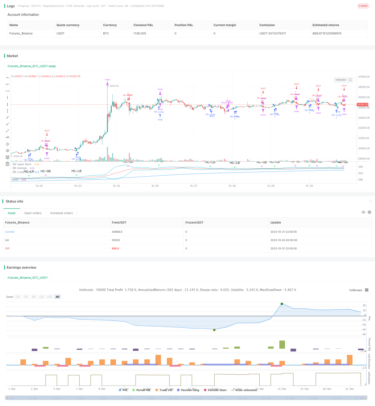
/*backtest
start: 2023-10-02 00:00:00
end: 2023-11-01 00:00:00
period: 1h
basePeriod: 15m
exchanges: [{"eid":"Futures_Binance","currency":"BTC_USDT"}]
*/

//@version=4

// This source code is subject to the terms of the Mozilla Public License 2.0 at https://mozilla.org/MPL/2.0/
// © MakeMoneyCoESTB2020

//*********************Notes for continued work***************
//3) add a Table of contents to each section of code
//4) add candle stick pattern considerations to chart
//5) add an input value for DTE range to backtest
//7) add abilit to turn on/off MACD plot
//9)
//************************************************************


//Hello my fellow investors
//After hours of reading, backtesting, and YouTube video watching
//I discovered that 200EMA, VWAP, BB, MACD, and STC 
//produce the most consistent results for investment planning.
//This strategy allows you to pick between the aforementioned indicators or layer them together.
//It works on the pricipal of:
//1) Always follow the market trend - buy/sell above/below 200EMA
//2) Follow corporate investing trends - buy/sell above/below VWAP
//3) Apply MACD check - buy--> MACD line above signal line 
// and corssover below histogram \\ sell --> MACD line below signal line 
// and crossover above histogram.
//4) Check volitility with price against BB limits upper/Sell or lower/buy
//5) When STC crosses about 10 buy and when it drops below 90 sell
//6) Exit position when stop loss is triggered or profit target is hit.  BB also provides a parameter to exit positions.

//This code is the product of many hours of hard work on the part of the greater tradingview community.  The credit goes to everyone in the community who has put code out there for the greater good.

//Happy Hunting!



//Title
// strategy("WOMBO COMBO: 100/200EMA & VWAP & MACD", shorttitle="WOMBO COMBO", default_qty_type=strategy.percent_of_equity, default_qty_value=1.5, initial_capital=10000,slippage=2, currency=currency.USD, overlay=true)

//define calculations price source
price = input(title="Price Source", defval=close)


//***************************
//Calculate 20/50/100/200EMA 
EMAlength = input(title="EMA_Length", defval=200)
EMA=ema(price, EMAlength)
//plot EMA
ColorEMA=EMAlength==200?color.blue:EMAlength==100?color.aqua:EMAlength==50?color.orange:color.red
plot(EMA, title = "EMA", color = ColorEMA)


//*****************************
//calculate VWAP
ColorVWAP = (price > vwap) ? color.lime : color.maroon
plot(vwap, title = "VWAP", color=ColorVWAP, linewidth=2)


//*****************************
//calculate MACD
//define variables for speed
fast = 12, slow = 26
//define parameters to calculate MACD
fastMA = ema(price, fast)
slowMA = ema(price, slow)
//define MACD line
macd = fastMA - slowMA
//define SIGNAL line
signal = sma(macd, 9)
//plot MACD line
//plot(macd, title = "MACD",  color=color.orange)
//plot signal line
//plot(signal, title = "Signal", color=color.purple)
//plot histogram
//define histogram colors
//col_grow_above = color.green
//col_grow_below = color.red
//col_fall_above = color.lime
//col_fall_below = color.maroon
//define histogram value
//hist = macd - signal
//plot histogram
//plot(hist, title="Histogram", style=plot.style_columns, color=(hist>=0 ? (hist[1] < hist ? col_grow_above : col_fall_above) : (hist[1] < hist ? col_grow_below : col_fall_below) ), transp=0 )


//***************************************
//Calculate Bollinger Bands
//Define BB input variables
//lengthBB = input(20, minval=1)
//multBB = input(2.0, minval=0.001, maxval=50)
lengthBB = 20
multBB = 2
//define BB average
basisBB = sma(price, lengthBB)
//define BB standar deviation
devBB = multBB * stdev(price, lengthBB)
//define BB upper and lower limits
upperBB = basisBB + devBB
lowerBB = basisBB - devBB
//Plot BB graph
ShowBB = input(title="Show BB", defval="Y", type=input.string, options=["Y", "N"])
transP = (ShowBB=="Y") ? 0 : 100
plot (upperBB, title = "BB Upper Band", color = color.aqua, transp=transP)
plot (basisBB, title = "BB Average", color = color.red, transp=transP)
plot (lowerBB, title = "BB Lower Band", color = color.aqua, transp=transP)


//*************************************************
//Calculate STC
//fastLength = input(title="MACD Fast Length", type=input.integer, defval=12)
//slowLength = input(title="MACD Slow Length", type=input.integer, defval=26)
fastLength = 23
slowLength = 50
cycleLength = input(title="Cycle Length", type=input.integer, defval=10)
//d1Length = input(title="1st %D Length", type=input.integer, defval=3)
//d2Length = input(title="2nd %D Length", type=input.integer, defval=3)
d1Length = 3
d2Length = 3
srcSTC = close

macdSTC = ema(srcSTC, fastLength) - ema(srcSTC, slowLength)
k = nz(fixnan(stoch(macdSTC, macdSTC, macdSTC, cycleLength)))
d = ema(k, d1Length)
kd = nz(fixnan(stoch(d, d, d, cycleLength)))
stc = ema(kd, d2Length)
stc := 	stc > 100 ? 100 : stc < 0 ? 0 : stc
upperSTC = input(title="Upper STC limit", defval=90)
lowerSTC = input( title="Lower STC limit", defval=10)

ma1length=35
ma1 = ema(close,ma1length)
ma2 = ema(close,EMAlength)

//STCbuy = crossover(stc, lowerSTC) and ma1>ma2 and close>ma1
//STCsell = crossunder(stc, upperSTC) and ma1<ma2 and close<ma1
STCbuy = crossover(stc, lowerSTC) 
STCsell = crossunder(stc, upperSTC) 




//*************************************************
//Candle stick patterns
//DojiSize = input(0.05, minval=0.01, title="Doji size")
//data=(abs(open - close) <= (high - low) * DojiSize)
//plotchar(data, title="Doji", text='Doji', color=color.white)

data2=(close[2] > open[2] and min(open[1], close[1]) > close[2] and open < min(open[1], close[1]) and close < open )
//plotshape(data2, title= "Evening Star", color=color.red, style=shape.arrowdown, text="Evening\nStar")

data3=(close[2] < open[2] and max(open[1], close[1]) < close[2] and open > max(open[1], close[1]) and close > open )
//plotshape(data3,  title= "Morning Star", location=location.belowbar, color=color.lime, style=shape.arrowup, text="Morning\nStar")

data4=(open[1] < close[1] and open > close[1] and high - max(open, close) >= abs(open - close) * 3 and min(close, open) - low <= abs(open - close))
//plotshape(data4, title= "Shooting Star", color=color.red, style=shape.arrowdown, text="Shooting\nStar")

data5=(((high - low)>3*(open -close)) and  ((close - low)/(.001 + high - low) > 0.6) and ((open - low)/(.001 + high - low) > 0.6))
//plotshape(data5, title= "Hammer", location=location.belowbar, color=color.white, style=shape.diamond, text="H")

data5b=(((high - low)>3*(open -close)) and  ((high - close)/(.001 + high - low) > 0.6) and ((high - open)/(.001 + high - low) > 0.6))
//plotshape(data5b, title= "Inverted Hammer", location=location.belowbar, color=color.white, style=shape.diamond, text="IH")

data6=(close[1] > open[1] and open > close and open <= close[1] and open[1] <= close and open - close < close[1] - open[1] )
//plotshape(data6, title= "Bearish Harami",  color=color.red, style=shape.arrowdown, text="Bearish\nHarami")

data7=(open[1] > close[1] and close > open and close <= open[1] and close[1] <= open and close - open < open[1] - close[1] )
//plotshape(data7,  title= "Bullish Harami", location=location.belowbar, color=color.lime, style=shape.arrowup, text="Bullish\nHarami")

data8=(close[1] > open[1] and open > close and open >= close[1] and open[1] >= close and open - close > close[1] - open[1] )
//plotshape(data8,  title= "Bearish Engulfing", color=color.red, style=shape.arrowdown, text="Bearish\nEngulfing")

data9=(open[1] > close[1] and close > open and close >= open[1] and close[1] >= open and close - open > open[1] - close[1] )
//plotshape(data9, title= "Bullish Engulfing", location=location.belowbar, color=color.lime, style=shape.arrowup, text="Bullish\nEngulfling")

upper = highest(10)[1]
data10=(close[1] < open[1] and  open < low[1] and close > close[1] + ((open[1] - close[1])/2) and close < open[1])
//plotshape(data10, title= "Piercing Line", location=location.belowbar, color=color.lime, style=shape.arrowup, text="Piercing\nLine")

lower = lowest(10)[1]
data11=(low == open and  open < lower and open < close and close > ((high[1] - low[1]) / 2) + low[1])
//plotshape(data11, title= "Bullish Belt", location=location.belowbar, color=color.lime, style=shape.arrowup, text="Bullish\nBelt")

data12=(open[1]>close[1] and open>=open[1] and close>open)
//plotshape(data12, title= "Bullish Kicker", location=location.belowbar, color=color.lime, style=shape.arrowup, text="Bullish\nKicker")

data13=(open[1]<close[1] and open<=open[1] and close<=open)
//plotshape(data13, title= "Bearish Kicker", color=color.red, style=shape.arrowdown, text="Bearish\nKicker")

data14=(((high-low>4*(open-close))and((close-low)/(.001+high-low)>=0.75)and((open-low)/(.001+high-low)>=0.75)) and high[1] < open and high[2] < open)
//plotshape(data14,  title= "Hanging Man", color=color.red, style=shape.arrowdown, text="Hanging\nMan")

data15=((close[1]>open[1])and(((close[1]+open[1])/2)>close)and(open>close)and(open>close[1])and(close>open[1])and((open-close)/(.001+(high-low))>0.6))
//plotshape(data15, title= "Dark Cloud Cover", color=color.red, style=shape.arrowdown, text="Dark\nCloudCover")




//**********Long & Short Entry Calculations***********************************
//Define countback variable
countback=input(minval=0, maxval=5, title="Price CountBack", defval=0)
//User input for what evaluations to run: EMA, VWAP, MACD, BB
EMA_Y_N=input(defval = "N", title="Run EMA", type=input.string, options=["Y", "N"])
VWAP_Y_N=input(defval = "N", title="Run VWAP", type=input.string, options=["Y", "N"])
MACD_Y_N=input(defval = "N", title="Run MACD", type=input.string, options=["Y", "N"])
BB_Y_N=input(defval = "N", title="Run BB", type=input.string, options=["Y", "N"])
STC_Y_N=input(defval = "Y", title="Run STC", type=input.string, options=["Y", "N"])
//long entry condition
dataHCLB=(iff(STC_Y_N=="Y", STCbuy, true) and iff(EMA_Y_N=="Y", price[countback]>EMA, true) and iff(VWAP_Y_N=="Y", price[countback]>vwap, true) and iff(MACD_Y_N=="Y", crossunder(signal[countback], macd[countback]), true) and iff(MACD_Y_N=="Y", macd[countback]<0, true) and iff(BB_Y_N=="Y", crossunder(price[countback], lowerBB), true))
plotshape(dataHCLB, title= "HC-LB", color=color.lime, style=shape.circle, text="HC-LB")
strategy.entry("HC-Long", strategy.long, comment="HC-Long", when = dataHCLB)
//short entry condition
dataHCSB=(iff(STC_Y_N=="Y", STCsell, true) and iff(EMA_Y_N=="Y", price[countback]<EMA, true) and iff(VWAP_Y_N=="Y", price[countback]<vwap, true) and iff(MACD_Y_N=="Y", crossunder(macd[countback], signal[countback]), true) and iff(MACD_Y_N=="Y", signal[countback]>0, true) and iff(BB_Y_N=="Y", crossover(price[countback], upperBB), true))
plotshape(dataHCSB, title= "HC-SB", color=color.fuchsia, style=shape.circle, text="HC-SB")
strategy.entry("HC-Short", strategy.short, comment="HC-Short", when=dataHCSB)




//******************Exit Conditions******************************
// Profit and Loss Exit Calculations
// User Options to Change Inputs (%)
stopPer = input(5, title='Stop Loss %', type=input.float) / 100
takePer = input(10, title='Take Profit %', type=input.float) / 100

// Determine where you've entered and in what direction
longStop = strategy.position_avg_price * (1 - stopPer)
shortStop = strategy.position_avg_price * (1 + stopPer)
shortTake = strategy.position_avg_price * (1 - takePer)
longTake = strategy.position_avg_price * (1 + takePer)

//exit position conditions and orders
if strategy.position_size > 0 or crossunder(price[countback], upperBB)
    strategy.exit(id="Close Long", stop=longStop, limit=longTake)
if strategy.position_size < 0 or crossover(price[countback], lowerBB)
    strategy.exit(id="Close Short", stop=shortStop, limit=shortTake)

Mais.