Estratégia de Rastreamento de Momentum Adaptativo Multifatorial


Data de criação: 2023-12-12 12:02:13 última modificação: 2023-12-12 12:02:13
cópia: 0 Cliques: 648
1
focar em
1621
Seguidores

Estratégia de Rastreamento de Momentum Adaptativo Multifatorial

Visão geral

A estratégia de rastreamento de dinâmica de adaptação multifatorial permite a negociação automatizada de ativos altamente voláteis, como criptomoedas, por meio da integração de vários indicadores técnicos para identificar tendências de mercado e resistências de suporte crítico. A estratégia usa indicadores como RSI, MACD e Stochastic para determinar o momento certo de compra e venda, além de permitir a identificação de tendências mais precisas em combinação com a porcentagem de mudança de preço.

Princípio da estratégia

O núcleo da estratégia de rastreamento de dinâmica de adaptação de múltiplos fatores está na utilização integrada de vários indicadores técnicos. A estratégia usa principalmente os seguintes componentes:

  1. O indicador RSI determina sobrecompra e sobrevenda. Em combinação com diferentes parâmetros, pode-se identificar um sinal RSI comum ou um sinal RSI de Conner melhorado para determinar se há oportunidade de reversão.

  2. Os indicadores MACD ajudam a determinar a direção da tendência. Quando o MACD atravessa a linha de sinal ou a linha de sinal, gera sinais de compra e venda.

  3. O indicador estocástico identifica a zona de sobrevenda e sobrecompra. A linha K e a linha D do furo-morto combinado do furo-morto determinam se o sinal é invertido.

  4. A porcentagem de variação de preço é usada para verificar se uma ruptura é verdadeira. A porcentagem de variação de preços, como o preço mais alto, o preço mais baixo e o preço de fechamento em um determinado período, é calculada para determinar se uma ruptura é verdadeira.

  5. O indicador EMA julga o excesso de espaço em grandes níveis. A linha rápida atravessa a linha lenta como um sinal otimista e a linha baixa como um sinal pessimista.

A estratégia de optar por fazer mais de negociação de acordo com o mercado de vazio, e depois de entrar em posição, definir um stop loss para controlar eficazmente o risco. Quando o sinal de reversão aparece, optar por sair da posição. Todo o processo de decisão combina plenamente vários fatores de julgamento, permitindo um julgamento mais preciso.

Análise de vantagens

A estratégia tem as seguintes vantagens:

  1. A condução de múltiplos fatores tem uma vantagem de julgamento. Em comparação com um único indicador, o conjunto de indicadores múltiplos pode ser verificado entre si, tornando os resultados mais precisos e confiáveis, economizando custos de transação desnecessários.

  2. Condições rigorosas para evitar transações erradas. A estratégia estabelece requisitos rígidos para as condições de compra e venda, exigindo que vários indicadores liberem sinais ao mesmo tempo, de modo a filtrar o ruído e evitar transações erradas.

  3. Adaptação automática dos superparâmetros reduz a intervenção humana. Capacidade de calcular dinamicamente os parâmetros indicadores da estratégia embutida, evitando a subjetividade da escolha manual dos superparâmetros, tornando os Parâmetros da estratégia mais objetivos e científicos.

  4. A estratégia calcula e mapeia a posição de parada de perda em tempo real após a abertura da posição, o que permite controlar efetivamente os prejuízos individuais e evitar a ocorrência de rupturas.

Análise de Riscos

A estratégia também apresenta alguns riscos que devem ser evitados:

  1. A probabilidade de um indicador emitir um sinal errado. Embora a verificação de vários indicadores possa reduzir significativamente o índice de sinais errados, existe a possibilidade de que isso aconteça. Isso pode causar prejuízos desnecessários.

  2. Risco de ruptura do stop loss. Em casos extremos, o preço pode cair em um precipício, levando o stop loss original a ser facilmente quebrado, causando maiores perdas.

  3. A otimização excessiva dos parâmetros. Embora os parâmetros dinâmicos evitem a subjetividade da seleção artificial, eles também podem levar à otimização excessiva dos parâmetros e à perda de generalização.

Resolução:

  1. Aumentar a rigidez das condições de filtragem de sinais e reduzir a taxa de falhas.
  2. A construção de armazéns por lotes evita perdas excessivas.
  3. Aumentar a quantidade de amostras de teste e avaliar rigorosamente a estabilidade dos parâmetros.

Direção de otimização da estratégia

A estratégia de rastreamento de dinâmica de adaptação multifatorial também possui as seguintes dimensões de otimização:

  1. Aumentar o número de fatores de julgamento. Combinando mais diferentes tipos de julgamentos de sinais de indicadores, como a taxa de flutuação, o volume de transações e outros julgamentos auxiliares.

  2. Algoritmos para otimizar o mecanismo de parada. Algoritmos de parada mais avançados, como parada de rastreamento e parada de choque, podem ser introduzidos para reduzir ainda mais a probabilidade de quebra de parada.

  3. Introdução de modelos de aprendizado de máquina. Modelagem de dados históricos usando modelos como RNN e LSTM para auxiliar na tomada de decisões de compra e venda.

  4. Integração de estratégias. A adoção de várias estratégias secundárias e a integração com métodos de aprendizagem integrada permitem obter um desempenho mais estável.

Resumir

A integração de estratégias de rastreamento de impulso de auto-adaptação de múltiplos fatores usa vários indicadores técnicos para identificar o momento de compra e venda. Em comparação com um único indicador, o julgamento da estratégia é mais preciso, enquanto os parâmetros embutidos se adaptam e o mecanismo de parada controla o risco. O próximo passo é a introdução de mais fatores de decisão auxiliares, algoritmos avançados de parada e métodos de aprendizado de máquina para aumentar ainda mais a eficácia da estratégia.
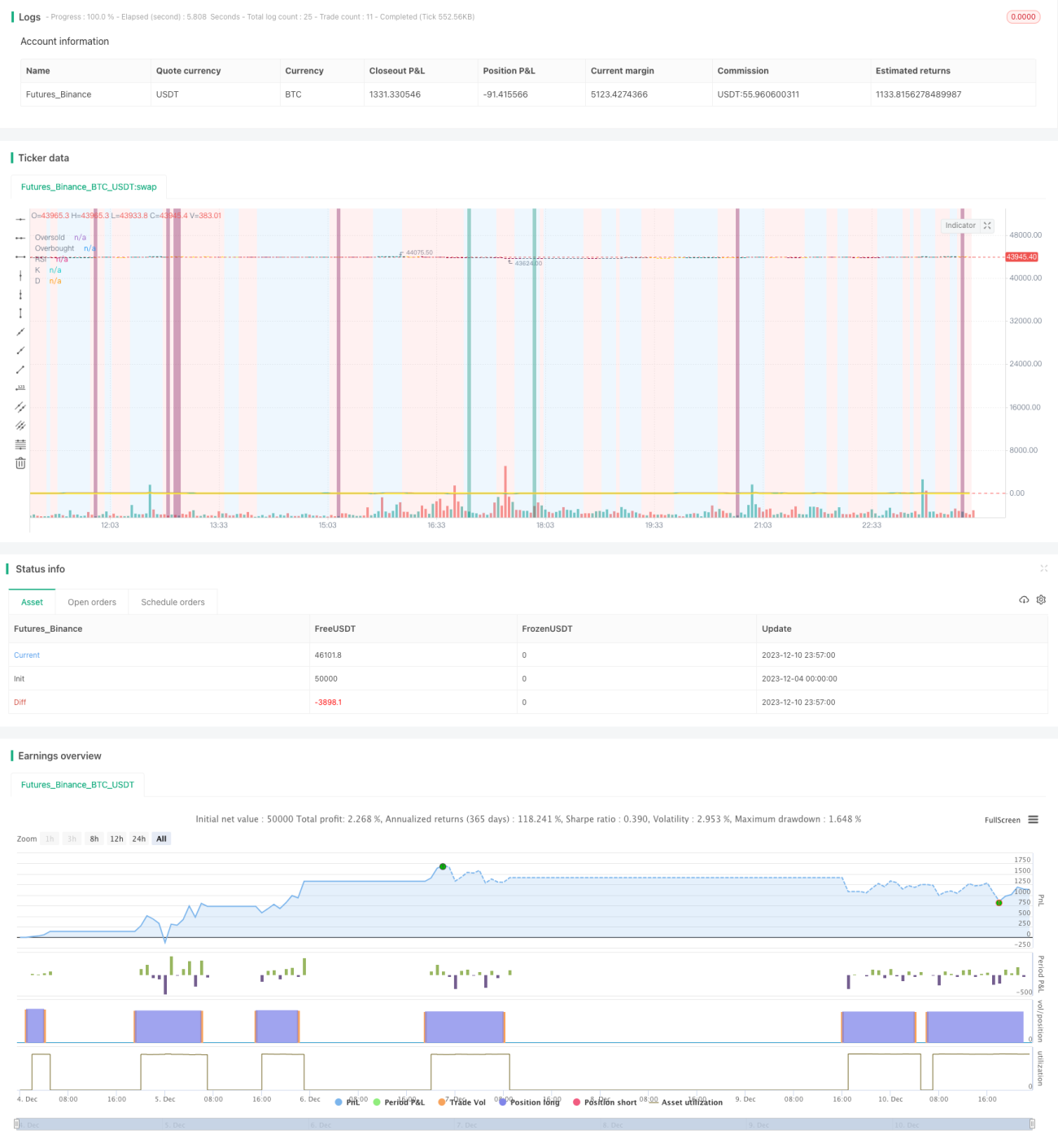
Código-fonte da estratégia
/*backtest
start: 2023-12-04 00:00:00
end: 2023-12-11 00:00:00
period: 3m
basePeriod: 1m
exchanges: [{"eid":"Futures_Binance","currency":"BTC_USDT"}]
*/

// This source code is subject to the terms of the Mozilla Public License 2.0 at https://mozilla.org/MPL/2.0/
//@version=4

// ██████╗██████╗ ███████╗ █████╗ ████████╗███████╗██████╗     ██████╗ ██╗   ██╗    
//██╔════╝██╔══██╗██╔════╝██╔══██╗╚══██╔══╝██╔════╝██╔══██╗    ██╔══██╗╚██╗ ██╔╝                       
//██║     ██████╔╝█████╗  ███████║   ██║   █████╗  ██║  ██║    ██████╔╝ ╚████╔╝                        
//██║     ██╔══██╗██╔══╝  ██╔══██║   ██║   ██╔══╝  ██║  ██║    ██╔══██╗  ╚██╔╝                         
//╚██████╗██║  ██║███████╗██║  ██║   ██║   ███████╗██████╔╝    ██████╔╝   ██║                          
// ╚═════╝╚═╝  ╚═╝╚══════╝╚═╝  ╚═╝   ╚═╝   ╚══════╝╚═════╝     ╚═════╝    ╚═╝                          
                                                                                                     
//███████╗ ██████╗ ██╗     ██╗   ██╗████████╗██╗ ██████╗ ███╗   ██╗███████╗ ██╗ █████╗ ███████╗ █████╗ 
//██╔════╝██╔═══██╗██║     ██║   ██║╚══██╔══╝██║██╔═══██╗████╗  ██║██╔════╝███║██╔══██╗╚════██║██╔══██╗
//███████╗██║   ██║██║     ██║   ██║   ██║   ██║██║   ██║██╔██╗ ██║███████╗╚██║╚██████║    ██╔╝╚█████╔╝
//╚════██║██║   ██║██║     ██║   ██║   ██║   ██║██║   ██║██║╚██╗██║╚════██║ ██║ ╚═══██║   ██╔╝ ██╔══██╗
//███████║╚██████╔╝███████╗╚██████╔╝   ██║   ██║╚██████╔╝██║ ╚████║███████║ ██║ █████╔╝   ██║  ╚█████╔╝
//╚══════╝ ╚═════╝ ╚══════╝ ╚═════╝    ╚═╝   ╚═╝ ╚═════╝ ╚═╝  ╚═══╝╚══════╝ ╚═╝ ╚════╝    ╚═╝   ╚════╝ 

strategy(shorttitle='Ain1 No Label',title='All in One Strategy no RSI Label', overlay=true, scale=scale.left, initial_capital = 1000, process_orders_on_close=true, default_qty_type = strategy.percent_of_equity, default_qty_value = 100, commission_type=strategy.commission.percent, commission_value=0.18, calc_on_every_tick=true)

kcolor = color.new(#0094FF, 60)
dcolor = color.new(#FF6A00, 60)


// -----------------  Strategy Inputs -------------------------------------------------------------
//Backtest dates with auto finish date of today
start = input(defval = timestamp("01 April 2021 00:00 -0500"), title = "Start Time", type = input.time)
finish = input(defval = timestamp("31 December 2021 00:00 -0600"), title = "End Time", type = input.time)
window()  => true       // create function "within window of time"


// Strategy Selection - Long, Short, or Both
stratinfo = input(true, "Long/Short for Mixed Market, Long for Bull, Short for Bear")
strat = input(title="Trade Types", defval="Long/Short", options=["Long Only", "Long/Short", "Short Only"])
strat_val = strat == "Long Only" ? 1 : strat == "Long/Short" ? 0 : -1

// Risk Management Inputs
sl= input(10.0, "Stop Loss %", minval = 0, maxval = 100, step = 0.01)
stoploss = sl/100
tp = input(20.0, "Target Profit %", minval = 0, maxval = 100, step = 0.01)
TargetProfit = tp/100


useXRSI = input(false, "Use RSI crossing back, select only one strategy")
useCRSI = input(false, "Use Tweaked Connors RSI, select only one")
RSIInfo = input(true, "These are the RSI Strategy Inputs, RSI Length applies to MACD, set OB and OS to 45 for using Stoch and EMA strategies.")
length = input(14, "RSI Length", minval=1)
overbought= input(62, "Overbought")
oversold= input(35, "Oversold")
cl1 = input(3, "Connor's MA Length 1", minval=1, step=1)
cl2 = input(20, "Connor's MA Lenght 2", minval=1, step=1)
cl3 = input(50, "Connor's MA Lenght 3", minval=1, step=1)

// MACD and EMA Inputs
useMACD = input(false, "Use MACD Only, select only one strategy")
useEMA  = input(false, "Use EMA Only, select only one strategy (EMA uses Stochastic inputs too)")
MACDInfo=input(true, "These are the MACD strategy variables")
fastLength = input(5, minval=1, title="EMA Fast Length")
slowLength = input(10, minval=1, title="EMA Slow Length")
ob_min = input(52, "Overbought Lookback Minimum Value", minval=0, maxval=200)
ob_lb = input(25, "Overbought Lookback Bars", minval=0, maxval=100)
os_min = input(50, "Oversold Lookback Minimum Value", minval=0, maxval=200)
os_lb = input(35, "Oversold Lookback Bars", minval=0, maxval=100)
source = input(title="Source", type=input.source, defval=close)
RSI = rsi(source, length)


// Price Movement Inputs
PriceInfo = input(true, "Price Change Percentage Cross Check Inputs for all Strategies, added logic to avoid early sell")
lkbk = input(5,"Max Lookback Period")

// EMA and SMA Background Inputs
useStoch    = input(false, "Use Stochastic Strategy, choose only one")
StochInfo   = input(true, "Stochastic Strategy Inputs")
smoothK     = input(3, "K", minval=1)
smoothD     = input(3, "D", minval=1)
k_mode      = input("SMA", "K Mode", options=["SMA", "EMA", "WMA"])
high_source = input(high,"High Source")
low_source= input(low,"Low Source")
HTF = input("","Curernt or Higher time frame only", type=input.resolution)

// Selections to show or hide the overlays
showZones = input(true, title="Show Bullish/Bearish Zones")
showStoch = input(true, title="Show Stochastic Overlays")
showRSIBS = input(true, title="Show RSI Buy Sell Zones")
showMACD = input(true, title="Show MACD")
color_bars=input(true, "Color Bars")


// ------------------ Dynamic RSI Calculation ----------------------------------------

AvgHigh(src,cnt,val) =>
    total = 0.0
    count = 0
    for i = 0 to cnt
        if src[i] > val
            count := count + 1
            total := total + src[i]
    round(total / count)
    
RSI_high = AvgHigh(RSI, ob_lb, ob_min)

AvgLow(src,cnt,val) =>
    total = 0.0
    count = 0
    for i = 0 to cnt
        if src[i] < val
            count := count + 1
            total := total + src[i]
    round(total / count)

RSI_low = AvgLow(RSI, os_lb, os_min)


// ------------------ Price Percentage Change Calculation -----------------------------------------
perc_change(lkbk) =>
    overall_change = ((close[0] - open[lkbk]) / open[lkbk]) * 100
    highest_high = 0.0
    lowest_low = 0.0
    for i = lkbk to 0
        highest_high := i == lkbk ? high : high[i] > high[(i + 1)] ? high[i] : highest_high[1]
        lowest_low := i == lkbk ? low : low[i] < low[(i + 1)] ? low[i] : lowest_low[1]
    
    start_to_high = ((highest_high - open[lkbk]) / open[lkbk]) * 100
    start_to_low = ((lowest_low - open[lkbk]) / open[lkbk]) * 100
    previous_to_high = ((highest_high - open[1])/open[1])*100
    previous_to_low = ((lowest_low-open[1])/open[1])*100
    previous_bar = ((close[1]-open[1])/open[1])*100
    
    [overall_change, start_to_high, start_to_low, previous_to_high, previous_to_low, previous_bar]
    
// Call the function    
[overall, to_high, to_low, last_high, last_low, last_bar] = perc_change(lkbk)

// Plot the function
//plot(overall*50, color=color.white, title='Overall Percentage Change', linewidth=3)
//plot(to_high*50, color=color.green,title='Percentage Change from Start to High', linewidth=2)
//plot(to_low*50, color=color.red, title='Percentage Change from Start to Low', linewidth=2)
//plot(last_high*100, color=color.teal, title="Previous to High", linewidth=2)
//plot(last_low*100, color=color.maroon, title="Previous to Close", linewidth=2)
//plot(last_bar*100, color=color.orange, title="Previous Bar", linewidth=2)
//hline(0, title='Center Line', color=color.orange, linewidth=2)

true_dip = overall < 0 and to_high > 0 and to_low < 0 and last_high > 0 and last_low < 0 and last_bar < 0
true_peak = overall > 0 and to_high > 0 and to_low > 0 and last_high > 0 and last_low < 0 and last_bar > 0

alertcondition(true_dip, title='True Dip', message='Dip')
alertcondition(true_peak, title='True Peak', message='Peak')

// ------------------ Background Colors based on EMA Indicators -----------------------------------
// Uses standard lengths of 9 and 21, if you want control delete the constant definition and uncomment the inputs
haClose(gap) => (open[gap] + high[gap] + low[gap] + close[gap]) / 4
rsi_ema = rsi(haClose(0), length)
v2 = ema(rsi_ema, length)                                                
v3 = 2 * v2 - ema(v2, length)  
emaA = ema(rsi_ema, fastLength)                                     
emaFast = 2 * emaA - ema(emaA, fastLength)
emaB = ema(rsi_ema, slowLength)                                     
emaSlow = 2 * emaB - ema(emaB, slowLength) 

//plot(rsi_ema, color=color.white, title='RSI EMA', linewidth=3)
//plot(v2, color=color.green,title='v2', linewidth=2)
//plot(v3, color=color.red, title='v3', linewidth=2)
//plot(emaFast, color=color.teal, title="EMA Fast", linewidth=2)
//plot(emaSlow, color=color.maroon, title="EMA Slow", linewidth=2)

EMABuy = crossunder(emaFast, v2) and window()
EMASell = crossover(emaFast, emaSlow) and window()


alertcondition(EMABuy, title='EMA Buy', message='EMA Buy Condition')
alertcondition(EMASell, title='EMA Sell', message='EMA Sell Condition')


// bullish signal rule: 
bullishRule =emaFast > emaSlow
// bearish signal rule: 
bearishRule =emaFast < emaSlow

// current trading State
ruleState = 0
ruleState := bullishRule ? 1 : bearishRule ? -1 : nz(ruleState[1])
ruleColor = ruleState==1 ? color.new(color.blue, 90) : ruleState == -1 ? color.new(color.red, 90) : ruleState == 0 ? color.new(color.gray, 90) : na
bgcolor(showZones ? ruleColor : na, title="Bullish/Bearish Zones")


// ------------------  Stochastic Indicator Overlay -----------------------------------------------

// Calculation
// Use highest highs and lowest lows
h_high = highest(high_source ,lkbk)
l_low = lowest(low_source ,lkbk)

stoch = stoch(RSI, RSI_high, RSI_low, length)
k =
 k_mode=="EMA" ? ema(stoch, smoothK) :
 k_mode=="WMA" ? wma(stoch, smoothK) :
 sma(stoch, smoothK)
d = sma(k, smoothD)
k_c = change(k)
d_c = change(d)
kd = k - d

// Plot
signalColor = k>oversold and d<overbought and k>d and k_c>0 and d_c>0 ? kcolor : 
 k<overbought and d>oversold and k<d and k_c<0 and d_c<0 ? dcolor : na
kp = plot(showStoch ? k : na, "K", color=kcolor)
dp = plot(showStoch ? d : na, "D", color=dcolor)
fill(kp, dp, color = signalColor, title="K-D")
signalUp = showStoch ? not na(signalColor) and kd>0 : na
signalDown = showStoch ? not na(signalColor) and kd<0 : na
//plot(signalUp ? kd : na, "Signal Up", color=kcolor, transp=90, style=plot.style_columns)
//plot(signalDown ? (kd+100) : na , "Signal Down", color=dcolor, transp=90, style=plot.style_columns, histbase=100)

//StochBuy = crossover(k, d) and kd>0 and to_low<0 and window()
//StochSell = crossunder(k,d) and kd<0 and to_high>0 and window()

StochBuy = crossover(k, d) and window()
StochSell = crossunder(k, d) and window()

alertcondition(StochBuy, title='Stoch Buy', message='K Crossing D')
alertcondition(StochSell, title='Stoch Sell', message='D Crossing K')


// -------------- Add Price Movement -------------------------
// Calculations
h1 = vwma(high, length)
l1 = vwma(low, length)
hp = h_high[1]
lp = l_low[1]

// Plot
var plot_color=#353535
var sig = 0
if (h1 >hp)
    sig:=1
    plot_color:=color.lime
else if (l1 <lp)
    sig:=-1
    plot_color:=color.maroon
//plot(1,title = "Price Movement Bars", style=plot.style_columns,color=plot_color)
//plot(sig,title="Signal 1 or -1",display=display.none)


// --------------------------------------- RSI Plot ----------------------------------------------
// Plot Oversold and Overbought Lines
over = hline(oversold, title="Oversold", color=color.green)
under = hline(overbought, title="Overbought", color=color.red)
fillcolor = color.new(#9915FF, 90)
fill(over, under, fillcolor, title="Band Background")


// Show RSI and EMA crosses with arrows and RSI Color (tweaked Connors RSI)
// Improves strategy setting ease by showing where EMA 5 crosses EMA 10 from above to confirm overbought conditions or trend reversals
// This shows where you should enter shorts or exit longs

// Tweaked Connors RSI Calculation
connor_ob = overbought
connor_os = oversold
ma1 = sma(close,cl1)
ma2 = sma(close, cl2)
ma3 = sma(close, cl3)

// Buy Sell Zones using tweaked Connors RSI (RSI values of 80 and 20 for Crypto as well as ma3, ma20, and ma50 are the tweaks)
RSI_SELL = ma1 > ma2 and open > ma3 and RSI >= connor_ob and true_peak and window()
RSI_BUY = ma2 < ma3 and ma3 > close and RSI <= connor_os and true_dip and window()

alertcondition(RSI_BUY, title='Connors Buy', message='Connors RSI Buy')
alertcondition(RSI_SELL, title='Connors Sell', message='Connors RSI Sell')

// Color Definition
col = useCRSI ? (close > ma2 and close < ma3 and RSI <= connor_os ? color.lime : close < ma2 and close > ma3 and RSI <= connor_ob ? color.red : color.yellow ) : color.yellow

// Plot colored RSI Line
plot(RSI, title="RSI", linewidth=3, color=col)


//------------------- MACD Strategy -------------------------------------------------
[macdLine, signalLine, _] = macd(close, fastLength, slowLength, length)

bartrendcolor = macdLine > signalLine and k > 50 and RSI > 50 ? color.teal : macdLine < signalLine and k < 50 and RSI < 50 ? color.maroon : macdLine < signalLine ? color.yellow : color.gray
barcolor(color = color_bars ? bartrendcolor : na)


MACDBuy = macdLine>signalLine and RSI<RSI_low and overall<0 and window()
MACDSell = macdLine<signalLine and RSI>RSI_high and overall>0 and window()

//plotshape(showMACD ? MACDBuy: na, title = "MACD Buy", style = shape.arrowup, text = "MACD Buy", color=color.green, textcolor=color.green, size=size.small)
//plotshape(showMACD ? MACDSell: na, title = "MACD Sell", style = shape.arrowdown, text = "MACD Sell", color=color.red, textcolor=color.red, size=size.small)
MACColor = MACDBuy ? color.new(color.teal, 50) : MACDSell ? color.new(color.maroon, 50) : na
bgcolor(showMACD ? MACColor : na, title ="MACD Signals")


// -------------------------------- Entry and Exit Logic ------------------------------------


// Entry Logic
XRSI_OB = crossunder(RSI, overbought) and overall<0 and window()
RSI_OB = RSI>overbought and true_peak and window()
XRSI_OS = crossover(RSI, oversold) and overall>0 and window()
RSI_OS = RSI<oversold and true_dip and window()

alertcondition(XRSI_OB, title='Reverse RSI Sell', message='RSI Crossing back under OB')
alertcondition(XRSI_OS, title='Reverse RSI Buy', message='RSI Crossing back over OS')

alertcondition(RSI_OS, title='RSI Buy', message='RSI Crossover OS')
alertcondition(RSI_SELL, title='RSI Sell', message='RSI Crossunder OB')


// Strategy Entry and Exit with built in Risk Management
GoLong = strategy.position_size==0 and strat_val > -1 and rsi_ema > RSI and k < d ? (useXRSI ? XRSI_OS : useMACD ? MACDBuy : useCRSI ? RSI_BUY : useStoch ? StochBuy : RSI_OS) : false

GoShort = strategy.position_size==0 and strat_val < 1 and rsi_ema < RSI and d < k ? (useXRSI ? XRSI_OB : useMACD ? MACDSell : useCRSI ? RSI_SELL : useStoch ? StochSell : RSI_OB) : false

if (GoLong)
    strategy.entry("LONG", strategy.long)

if (GoShort) 
    strategy.entry("SHORT", strategy.short)


longStopPrice  = strategy.position_avg_price * (1 - stoploss)
longTakePrice  = strategy.position_avg_price * (1 + TargetProfit)
shortStopPrice = strategy.position_avg_price * (1 + stoploss)
shortTakePrice = strategy.position_avg_price * (1 - TargetProfit)

//plot(series=(strategy.position_size > 0) ? longTakePrice : na, color=color.green, style=plot.style_circles, linewidth=3, title="Long Take Profit")
//plot(series=(strategy.position_size < 0) ? shortTakePrice : na, color=color.green, style=plot.style_circles, linewidth=3, title="Short Take Profit")
//plot(series=(strategy.position_size > 0) ? longStopPrice : na, color=color.red, style=plot.style_cross, linewidth=2, title="Long Stop Loss")
//plot(series=(strategy.position_size < 0) ? shortStopPrice : na, color=color.red, style=plot.style_cross, linewidth=2, title="Short Stop Loss")

if (strategy.position_size > 0)
    strategy.exit(id="Exit Long", from_entry = "LONG", stop = longStopPrice, limit = longTakePrice)
    
if (strategy.position_size < 0)
    strategy.exit(id="Exit Short", from_entry = "SHORT", stop = shortStopPrice, limit = shortTakePrice)


CloseLong = strat_val > -1 and strategy.position_size > 0 and rsi_ema > RSI and d > k ? (useXRSI ? XRSI_OB : useMACD ? MACDSell : useCRSI ? RSI_SELL : RSI_OB) : false

if(CloseLong)
    strategy.close("LONG")
        
CloseShort = strat_val < 1 and strategy.position_size < 0 and rsi_ema < RSI and k > d ? (useXRSI ? XRSI_OS : useMACD ? MACDBuy : useCRSI ? RSI_BUY : RSI_OS) : false

if(CloseShort)
    strategy.close("SHORT")