Estratégia de acompanhamento de tendências do canal gaussiano
Visão geral
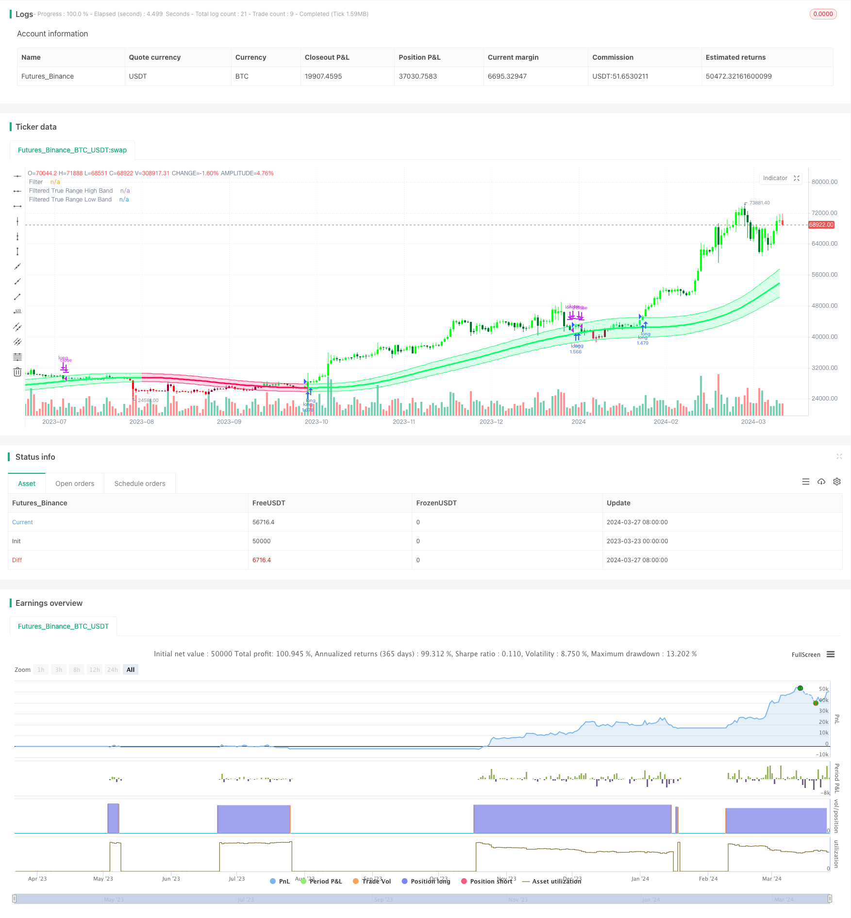
A estratégia de acompanhamento de tendências do canal gaussiano é uma estratégia de negociação de seguimento de tendências baseada no indicador do canal gaussiano. A estratégia visa capturar as principais tendências do mercado, comprando e mantendo posições em tendências ascendentes e observando posições em tendências descendentes. A estratégia usa o indicador do canal gaussiano para identificar a direção e a intensidade da tendência e determinar a hora de comprar e vender, analisando a relação entre o preço e a descida do canal.
Princípio da estratégia
No centro da estratégia de rastreamento de tendências do canal gaussiano está o indicador do canal gaussiano, proposto por Ehlers, uma ferramenta de análise de tendências que utiliza a técnica de Gauss e a combinação de True Range. O indicador primeiro calcula os valores β e α de acordo com o ciclo de amostragem e o número de pontos polares, e depois processa os dados em um filtro, obtendo uma curva de nivelamento.
Vantagens estratégicas
- Seguimento de tendências: A estratégia é boa para capturar as principais tendências do mercado e investir na direção das tendências, o que ajuda a obter um retorno estável a longo prazo.
- Redução da frequência de negociação: a estratégia só é adotada quando a tendência é confirmada, mantendo a posição enquanto a tendência persiste, reduzindo o número de negociações desnecessárias e os custos de negociação.
- Reduzir o atraso: reduzindo o atraso e o modo de resposta rápida, a estratégia pode reagir mais rapidamente às mudanças no mercado.
- Flexibilidade de parâmetros: O usuário pode ajustar os parâmetros da estratégia de acordo com suas necessidades, como o ciclo de amostragem, o número de pontos de polarização e o múltiplo do alcance real, para otimizar o desempenho da estratégia.
Risco estratégico
- Risco de otimização de parâmetros: configurações inadequadas de parâmetros podem levar a um mau desempenho da estratégia. É recomendável otimizar e testar os parâmetros em diferentes cenários de mercado para encontrar a melhor combinação de parâmetros.
- Risco de reversão de tendência: quando a tendência do mercado ocorre uma reversão súbita, a estratégia pode produzir um retorno maior. O risco pode ser controlado por meio da configuração de stop loss ou da introdução de outros indicadores.
- Risco de mercado de turbulência: Em mercados de turbulência, a estratégia pode apresentar sinais de negociação frequentes, resultando em prejuízos nos lucros. Os sinais podem ser filtrados por meio de parâmetros de otimização ou em combinação com outros indicadores técnicos.
Direção de otimização da estratégia
- Introdução de outros indicadores técnicos: em combinação com outros indicadores de tendência ou de oscilação, como MACD, RSI, etc., para melhorar a precisão e a confiabilidade do sinal.
- Otimização de parâmetros dinâmicos: ajuste dinâmico dos parâmetros da estratégia de acordo com as mudanças no estado do mercado para se adaptar a diferentes circunstâncias do mercado.
- Adição do módulo de controle de risco: configuração de regras razoáveis de stop loss e stop loss, controle do risco de cada transação e nível de retirada geral.
- Análise de múltiplos períodos de tempo: combina sinais de diferentes períodos de tempo, como a linha do dia, a linha de 4 horas, etc., para obter informações de mercado mais abrangentes.
Resumir
A estratégia de acompanhamento de tendências do canal gaussiano é uma estratégia de negociação de acompanhamento de tendências baseada na tecnologia de Gauss para obter lucros estáveis a longo prazo, capturando as principais tendências do mercado. A estratégia usa o indicador do canal gaussiano para identificar a direção e a intensidade da tendência, oferecendo ao mesmo tempo a capacidade de reduzir o atraso e a resposta rápida.
/*backtest
start: 2023-03-23 00:00:00
end: 2024-03-28 00:00:00
period: 1d
basePeriod: 1h
exchanges: [{"eid":"Futures_Binance","currency":"BTC_USDT"}]
*/

//@version=5
strategy(title="Gaussian Channel Strategy v2.0", overlay=true, calc_on_every_tick=false, initial_capital=1000, default_qty_type=strategy.percent_of_equity, default_qty_value=100, commission_type=strategy.commission.percent, commission_value=0.1, slippage=3)

//-----------------------------------------------------------------------------------------------------------------------------------------------------------------
// Gaussian Channel Indicaor - courtesy of @DonovanWall
//-----------------------------------------------------------------------------------------------------------------------------------------------------------------

// Date condition inputs
startDate = input(timestamp("1 January 2018 00:00 +0000"), "Date Start", group="Main Algo Settings")
endDate = input(timestamp("1 January 2060 00:00 +0000"), "Date Start", group="Main Algo Settings")
timeCondition = true

// This study is an experiment utilizing the Ehlers Gaussian Filter technique combined with lag reduction techniques and true range to analyze trend activity.
// Gaussian filters, as Ehlers explains it, are simply exponential moving averages applied multiple times.
// First, beta and alpha are calculated based on the sampling period and number of poles specified. The maximum number of poles available in this script is 9.
// Next, the data being analyzed is given a truncation option for reduced lag, which can be enabled with "Reduced Lag Mode".
// Then the alpha and source values are used to calculate the filter and filtered true range of the dataset.
// Filtered true range with a specified multiplier is then added to and subtracted from the filter, generating a channel.
// Lastly, a one pole filter with a N pole alpha is averaged with the filter to generate a faster filter, which can be enabled with "Fast Response Mode".

// Custom bar colors are included.

// Note: Both the sampling period and number of poles directly affect how much lag the indicator has, and how smooth the output is.
//      Larger inputs will result in smoother outputs with increased lag, and smaller inputs will have noisier outputs with reduced lag.
//      For the best results, I recommend not setting the sampling period any lower than the number of poles + 1. Going lower truncates the equation.

//-----------------------------------------------------------------------------------------------------------------------------------------------------------------
// Updates:
// Huge shoutout to @e2e4mfck for taking the time to improve the calculation method!
// -> migrated to v4
// -> pi is now calculated using trig identities rather than being explicitly defined.
// -> The filter calculations are now organized into functions rather than being individually defined.
// -> Revamped color scheme.

//-----------------------------------------------------------------------------------------------------------------------------------------------------------------
// Functions - courtesy of @e2e4mfck
//-----------------------------------------------------------------------------------------------------------------------------------------------------------------

// Filter function
f_filt9x (_a, _s, _i) =>
    int _m2 = 0, int _m3 = 0, int _m4 = 0, int _m5 = 0, int _m6 = 0,
    int _m7 = 0, int _m8 = 0, int _m9 = 0, float _f = .0, _x = (1 - _a)
    // Weights.
    // Initial weight _m1 is a pole number and equal to _i
    _m2 := _i == 9 ? 36  : _i == 8 ? 28 : _i == 7 ? 21 : _i == 6 ? 15 : _i == 5 ? 10 : _i == 4 ? 6 : _i == 3 ? 3 : _i == 2 ? 1 : 0
    _m3 := _i == 9 ? 84  : _i == 8 ? 56 : _i == 7 ? 35 : _i == 6 ? 20 : _i == 5 ? 10 : _i == 4 ? 4 : _i == 3 ? 1 : 0
    _m4 := _i == 9 ? 126 : _i == 8 ? 70 : _i == 7 ? 35 : _i == 6 ? 15 : _i == 5 ? 5  : _i == 4 ? 1 : 0
    _m5 := _i == 9 ? 126 : _i == 8 ? 56 : _i == 7 ? 21 : _i == 6 ? 6  : _i == 5 ? 1  : 0
    _m6 := _i == 9 ? 84  : _i == 8 ? 28 : _i == 7 ? 7  : _i == 6 ? 1  : 0
    _m7 := _i == 9 ? 36  : _i == 8 ? 8  : _i == 7 ? 1  : 0
    _m8 := _i == 9 ? 9   : _i == 8 ? 1  : 0
    _m9 := _i == 9 ? 1   : 0
    // filter
    _f :=   math.pow(_a, _i) * nz(_s) +
      _i  *     _x      * nz(_f[1])      - (_i >= 2 ?
      _m2 * math.pow(_x, 2)  * nz(_f[2]) : 0) + (_i >= 3 ?
      _m3 * math.pow(_x, 3)  * nz(_f[3]) : 0) - (_i >= 4 ?
      _m4 * math.pow(_x, 4)  * nz(_f[4]) : 0) + (_i >= 5 ?
      _m5 * math.pow(_x, 5)  * nz(_f[5]) : 0) - (_i >= 6 ?
      _m6 * math.pow(_x, 6)  * nz(_f[6]) : 0) + (_i >= 7 ?
      _m7 * math.pow(_x, 7)  * nz(_f[7]) : 0) - (_i >= 8 ?
      _m8 * math.pow(_x, 8)  * nz(_f[8]) : 0) + (_i == 9 ?
      _m9 * math.pow(_x, 9)  * nz(_f[9]) : 0)

// 9 var declaration fun
f_pole (_a, _s, _i) =>
    _f1 =            f_filt9x(_a, _s, 1),      _f2 = (_i >= 2 ? f_filt9x(_a, _s, 2) : 0), _f3 = (_i >= 3 ? f_filt9x(_a, _s, 3) : 0)
    _f4 = (_i >= 4 ? f_filt9x(_a, _s, 4) : 0), _f5 = (_i >= 5 ? f_filt9x(_a, _s, 5) : 0), _f6 = (_i >= 6 ? f_filt9x(_a, _s, 6) : 0)
    _f7 = (_i >= 2 ? f_filt9x(_a, _s, 7) : 0), _f8 = (_i >= 8 ? f_filt9x(_a, _s, 8) : 0), _f9 = (_i == 9 ? f_filt9x(_a, _s, 9) : 0)
    _fn = _i == 1 ? _f1 : _i == 2 ? _f2 : _i == 3 ? _f3 :
      _i == 4     ? _f4 : _i == 5 ? _f5 : _i == 6 ? _f6 :
      _i == 7     ? _f7 : _i == 8 ? _f8 : _i == 9 ? _f9 : na
    [_fn, _f1]

//-----------------------------------------------------------------------------------------------------------------------------------------------------------------
// Inputs
//-----------------------------------------------------------------------------------------------------------------------------------------------------------------

// Source
src = input(defval=hlc3, title="Source")

// Poles
int N = input.int(defval=4, title="Poles", minval=1, maxval=9)

// Period
int per = input.int(defval=144, title="Sampling Period", minval=2)

// True Range Multiplier
float mult = input.float(defval=1.414, title="Filtered True Range Multiplier", minval=0)

// Lag Reduction
bool modeLag  = input.bool(defval=false, title="Reduced Lag Mode")
bool modeFast = input.bool(defval=false, title="Fast Response Mode")

//-----------------------------------------------------------------------------------------------------------------------------------------------------------------
// Definitions
//-----------------------------------------------------------------------------------------------------------------------------------------------------------------

// Beta and Alpha Components
beta  = (1 - math.cos(4*math.asin(1)/per)) / (math.pow(1.414, 2/N) - 1)
alpha = - beta + math.sqrt(math.pow(beta, 2) + 2*beta)

// Lag
lag = (per - 1)/(2*N)

// Data
srcdata = modeLag ? src + (src - src[lag]) : src
trdata  = modeLag ? ta.tr(true) + (ta.tr(true) - ta.tr(true)[lag]) : ta.tr(true)

// Filtered Values
[filtn, filt1]     = f_pole(alpha, srcdata, N)
[filtntr, filt1tr] = f_pole(alpha, trdata,  N)

// Lag Reduction
filt   = modeFast ? (filtn + filt1)/2 : filtn
filttr = modeFast ? (filtntr + filt1tr)/2 : filtntr

// Bands
hband = filt + filttr*mult
lband = filt - filttr*mult

// Colors
color1   = #0aff68
color2   = #00752d
color3   = #ff0a5a
color4   = #990032
fcolor   = filt > filt[1] ? #0aff68 : filt < filt[1] ? #ff0a5a : #cccccc
barcolor = (src > src[1]) and (src > filt) and (src < hband) ? #0aff68 : (src > src[1]) and (src >= hband) ? #0aff1b : (src <= src[1]) and (src > filt) ? #00752d :
           (src < src[1]) and (src < filt) and (src > lband) ? #ff0a5a : (src < src[1]) and (src <= lband) ? #ff0a11 : (src >= src[1]) and (src < filt) ? #990032 : #cccccc

//-----------------------------------------------------------------------------------------------------------------------------------------------------------------
// Outputs
//-----------------------------------------------------------------------------------------------------------------------------------------------------------------

// Filter Plot
filtplot = plot(filt, title="Filter", color=fcolor, linewidth=3)

// Band Plots
hbandplot = plot(hband, title="Filtered True Range High Band", color=fcolor)
lbandplot = plot(lband, title="Filtered True Range Low Band", color=fcolor)

// Channel Fill
fill(hbandplot, lbandplot, title="Channel Fill", color=color.new(fcolor, 80))

// Bar Color
barcolor(barcolor)

longCondition = ta.crossover(close, hband) and timeCondition
closeAllCondition = ta.crossunder(close, hband) and timeCondition

if longCondition
    strategy.entry("long", strategy.long)

if closeAllCondition
    strategy.close("long")