Стратегия с использованием нескольких показателей для выявления переломных точек торговли в квантовой торговле

Автор:Чао Чжан, Дата: 2023-11-02 14:09:34
Тэги:

Обзор

Эта стратегия объединяет 5 основных индикаторов, включая EMA, VWAP, MACD, Bollinger Bands и Schaff Trend Cycle, для определения точек перелома, когда цена изменяется в пределах определенного диапазона, и генерирует сигналы купли и продажи. Преимущество этой стратегии заключается в гибкости объединения различных индикаторов на основе различных рыночных условий для снижения ложных сигналов и повышения рентабельности.

Логика стратегии

EMA оценивает общую направленность тренда, покупает только с трендом
VWAP оценивает денежный поток институтов, покупает только тогда, когда учреждения покупают
MACD оценивает краткосрочный тренд и изменение импульса, линия MACD перекрестный сигнал линия является сигнал покупки/продажи
Боллингерские полосы оценивают условия перекупления и перепродажи, выход цены из полос предполагает сигналы покупки/продажи
Schaff Trend Cycle оценивает краткосрочную структуру диапазона, превышение высоких/низких порогов предполагает сигналы покупки/продажи
Отправить ордера на покупку/продажу, когда все 5 индикаторов согласны с сигналом
Установка стоп-лосса и прибыли для оптимизации управления капиталом

Преимущества

Снижение ложных сигналов с использованием комбинации с несколькими индикаторами

Использование комбинации таких индикаторов, как EMA, VWAP, MACD, BB и STC, позволяет перекрестной проверке исключить ложные сигналы из любых отдельных индикаторов, повышая надежность.

Настраиваемые показатели

Возможность включения/выключения показателей позволяет комбинировать идеальные показатели для различных продуктов и рыночных условий, повышая адаптивность.

Оптимизированное управление капиталом

Стоп-лосс и прибыль позволяют ограничить потери от одной сделки и зафиксировать прибыль, что позволяет лучше управлять капиталом.

Ясная логика стратегии

Простые интуитивные индикаторы, используемые с подробными комментариями к коду, облегчают понимание и изменение логики общей стратегии.

Сильная практичность

Широко используемые индикаторы с разумной настройкой позволяют торговать в режиме реального времени с приличными результатами сразу без обширных оптимизаций.

Риски

Риск идентификации задержанного сигнала

EMA, MACD и т.д. отстают в определении изменений цен, что может привести к отсутствию оптимального времени входа.

Риск неправильной настройки параметров

Плохие параметры индикатора будут генерировать чрезмерные ложные сигналы и нарушать стратегию.

Нет гарантии выигрыша

Многоиндикаторная комбинация улучшает, но не гарантирует выигрышную ставку.

Стоп-потеря слишком плотная

Если стоп-лосс слишком жесткий, нормальные колебания цен могут быть остановлены, вызывая ненужные потери.

Возможности для расширения

Добавить модель ML для оценки надежности сигнала

Модель поезда для оценки многопоказательных сигналов на надежность, фильтрация ложных сигналов.

Добавление индикаторов импульса для идентификации накопления

Добавьте количественные показатели, такие как OBV, чтобы определить накопление цен, улучшая уверенность в точке покупки.

Оптимизировать логику стоп-лосса и прибыли

Исследование более подходящей логики остановки или получения прибыли для этой стратегии, чтобы лучше оптимизировать управление капиталом.

Оптимизация параметров

Провести более систематические обратные испытания для поиска оптимальных параметров для каждого показателя, улучшая надежность.

Добавить автоматическую торговлю

Подключение к торговому API для автоматического выполнения ордеров, что позволяет полностью автоматизировать выполнение стратегии без вмешательства.

Заключение

Эта стратегия сочетает в себе сильные стороны нескольких технических индикаторов с ясным логическим потоком и сильной практической ценностью. Она может служить дискреционной поддержкой решений торговли или прямой алгоритмической торговлей. Но для снижения риска и улучшения стабильности перед последовательной прибыльной живой торговлей необходимы оптимизация и настройка на основе конкретного продукта и рыночной среды.

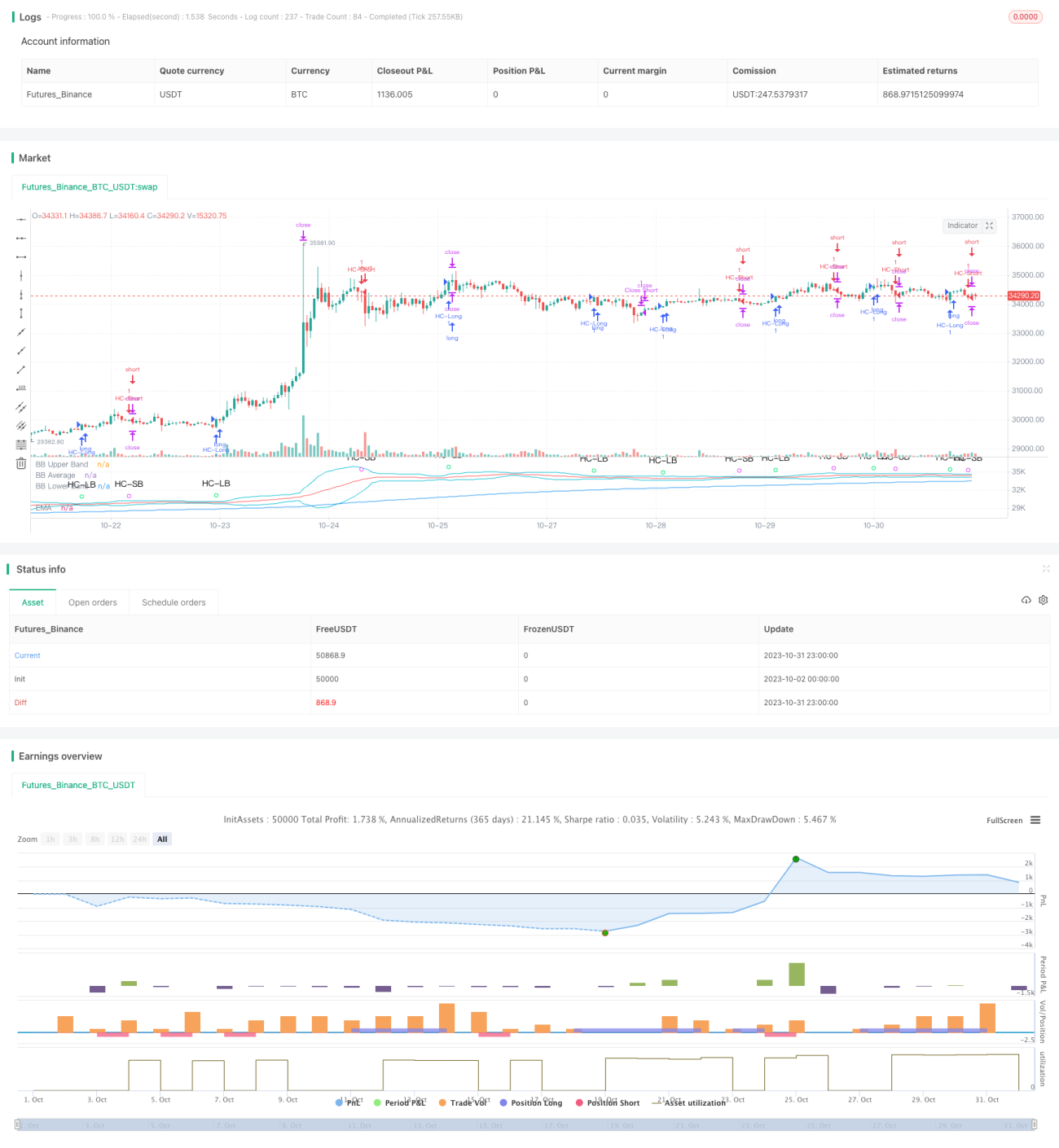
/*backtest
start: 2023-10-02 00:00:00
end: 2023-11-01 00:00:00
period: 1h
basePeriod: 15m
exchanges: [{"eid":"Futures_Binance","currency":"BTC_USDT"}]
*/

//@version=4

// This source code is subject to the terms of the Mozilla Public License 2.0 at https://mozilla.org/MPL/2.0/
// © MakeMoneyCoESTB2020

//*********************Notes for continued work***************
//3) add a Table of contents to each section of code
//4) add candle stick pattern considerations to chart
//5) add an input value for DTE range to backtest
//7) add abilit to turn on/off MACD plot
//9)
//************************************************************


//Hello my fellow investors
//After hours of reading, backtesting, and YouTube video watching
//I discovered that 200EMA, VWAP, BB, MACD, and STC 
//produce the most consistent results for investment planning.
//This strategy allows you to pick between the aforementioned indicators or layer them together.
//It works on the pricipal of:
//1) Always follow the market trend - buy/sell above/below 200EMA
//2) Follow corporate investing trends - buy/sell above/below VWAP
//3) Apply MACD check - buy--> MACD line above signal line 
// and corssover below histogram \\ sell --> MACD line below signal line 
// and crossover above histogram.
//4) Check volitility with price against BB limits upper/Sell or lower/buy
//5) When STC crosses about 10 buy and when it drops below 90 sell
//6) Exit position when stop loss is triggered or profit target is hit.  BB also provides a parameter to exit positions.

//This code is the product of many hours of hard work on the part of the greater tradingview community.  The credit goes to everyone in the community who has put code out there for the greater good.

//Happy Hunting!



//Title
// strategy("WOMBO COMBO: 100/200EMA & VWAP & MACD", shorttitle="WOMBO COMBO", default_qty_type=strategy.percent_of_equity, default_qty_value=1.5, initial_capital=10000,slippage=2, currency=currency.USD, overlay=true)

//define calculations price source
price = input(title="Price Source", defval=close)


//***************************
//Calculate 20/50/100/200EMA 
EMAlength = input(title="EMA_Length", defval=200)
EMA=ema(price, EMAlength)
//plot EMA
ColorEMA=EMAlength==200?color.blue:EMAlength==100?color.aqua:EMAlength==50?color.orange:color.red
plot(EMA, title = "EMA", color = ColorEMA)


//*****************************
//calculate VWAP
ColorVWAP = (price > vwap) ? color.lime : color.maroon
plot(vwap, title = "VWAP", color=ColorVWAP, linewidth=2)


//*****************************
//calculate MACD
//define variables for speed
fast = 12, slow = 26
//define parameters to calculate MACD
fastMA = ema(price, fast)
slowMA = ema(price, slow)
//define MACD line
macd = fastMA - slowMA
//define SIGNAL line
signal = sma(macd, 9)
//plot MACD line
//plot(macd, title = "MACD",  color=color.orange)
//plot signal line
//plot(signal, title = "Signal", color=color.purple)
//plot histogram
//define histogram colors
//col_grow_above = color.green
//col_grow_below = color.red
//col_fall_above = color.lime
//col_fall_below = color.maroon
//define histogram value
//hist = macd - signal
//plot histogram
//plot(hist, title="Histogram", style=plot.style_columns, color=(hist>=0 ? (hist[1] < hist ? col_grow_above : col_fall_above) : (hist[1] < hist ? col_grow_below : col_fall_below) ), transp=0 )


//***************************************
//Calculate Bollinger Bands
//Define BB input variables
//lengthBB = input(20, minval=1)
//multBB = input(2.0, minval=0.001, maxval=50)
lengthBB = 20
multBB = 2
//define BB average
basisBB = sma(price, lengthBB)
//define BB standar deviation
devBB = multBB * stdev(price, lengthBB)
//define BB upper and lower limits
upperBB = basisBB + devBB
lowerBB = basisBB - devBB
//Plot BB graph
ShowBB = input(title="Show BB", defval="Y", type=input.string, options=["Y", "N"])
transP = (ShowBB=="Y") ? 0 : 100
plot (upperBB, title = "BB Upper Band", color = color.aqua, transp=transP)
plot (basisBB, title = "BB Average", color = color.red, transp=transP)
plot (lowerBB, title = "BB Lower Band", color = color.aqua, transp=transP)


//*************************************************
//Calculate STC
//fastLength = input(title="MACD Fast Length", type=input.integer, defval=12)
//slowLength = input(title="MACD Slow Length", type=input.integer, defval=26)
fastLength = 23
slowLength = 50
cycleLength = input(title="Cycle Length", type=input.integer, defval=10)
//d1Length = input(title="1st %D Length", type=input.integer, defval=3)
//d2Length = input(title="2nd %D Length", type=input.integer, defval=3)
d1Length = 3
d2Length = 3
srcSTC = close

macdSTC = ema(srcSTC, fastLength) - ema(srcSTC, slowLength)
k = nz(fixnan(stoch(macdSTC, macdSTC, macdSTC, cycleLength)))
d = ema(k, d1Length)
kd = nz(fixnan(stoch(d, d, d, cycleLength)))
stc = ema(kd, d2Length)
stc := 	stc > 100 ? 100 : stc < 0 ? 0 : stc
upperSTC = input(title="Upper STC limit", defval=90)
lowerSTC = input( title="Lower STC limit", defval=10)

ma1length=35
ma1 = ema(close,ma1length)
ma2 = ema(close,EMAlength)

//STCbuy = crossover(stc, lowerSTC) and ma1>ma2 and close>ma1
//STCsell = crossunder(stc, upperSTC) and ma1<ma2 and close<ma1
STCbuy = crossover(stc, lowerSTC) 
STCsell = crossunder(stc, upperSTC) 




//*************************************************
//Candle stick patterns
//DojiSize = input(0.05, minval=0.01, title="Doji size")
//data=(abs(open - close) <= (high - low) * DojiSize)
//plotchar(data, title="Doji", text='Doji', color=color.white)

data2=(close[2] > open[2] and min(open[1], close[1]) > close[2] and open < min(open[1], close[1]) and close < open )
//plotshape(data2, title= "Evening Star", color=color.red, style=shape.arrowdown, text="Evening\nStar")

data3=(close[2] < open[2] and max(open[1], close[1]) < close[2] and open > max(open[1], close[1]) and close > open )
//plotshape(data3,  title= "Morning Star", location=location.belowbar, color=color.lime, style=shape.arrowup, text="Morning\nStar")

data4=(open[1] < close[1] and open > close[1] and high - max(open, close) >= abs(open - close) * 3 and min(close, open) - low <= abs(open - close))
//plotshape(data4, title= "Shooting Star", color=color.red, style=shape.arrowdown, text="Shooting\nStar")

data5=(((high - low)>3*(open -close)) and  ((close - low)/(.001 + high - low) > 0.6) and ((open - low)/(.001 + high - low) > 0.6))
//plotshape(data5, title= "Hammer", location=location.belowbar, color=color.white, style=shape.diamond, text="H")

data5b=(((high - low)>3*(open -close)) and  ((high - close)/(.001 + high - low) > 0.6) and ((high - open)/(.001 + high - low) > 0.6))
//plotshape(data5b, title= "Inverted Hammer", location=location.belowbar, color=color.white, style=shape.diamond, text="IH")

data6=(close[1] > open[1] and open > close and open <= close[1] and open[1] <= close and open - close < close[1] - open[1] )
//plotshape(data6, title= "Bearish Harami",  color=color.red, style=shape.arrowdown, text="Bearish\nHarami")

data7=(open[1] > close[1] and close > open and close <= open[1] and close[1] <= open and close - open < open[1] - close[1] )
//plotshape(data7,  title= "Bullish Harami", location=location.belowbar, color=color.lime, style=shape.arrowup, text="Bullish\nHarami")

data8=(close[1] > open[1] and open > close and open >= close[1] and open[1] >= close and open - close > close[1] - open[1] )
//plotshape(data8,  title= "Bearish Engulfing", color=color.red, style=shape.arrowdown, text="Bearish\nEngulfing")

data9=(open[1] > close[1] and close > open and close >= open[1] and close[1] >= open and close - open > open[1] - close[1] )
//plotshape(data9, title= "Bullish Engulfing", location=location.belowbar, color=color.lime, style=shape.arrowup, text="Bullish\nEngulfling")

upper = highest(10)[1]
data10=(close[1] < open[1] and  open < low[1] and close > close[1] + ((open[1] - close[1])/2) and close < open[1])
//plotshape(data10, title= "Piercing Line", location=location.belowbar, color=color.lime, style=shape.arrowup, text="Piercing\nLine")

lower = lowest(10)[1]
data11=(low == open and  open < lower and open < close and close > ((high[1] - low[1]) / 2) + low[1])
//plotshape(data11, title= "Bullish Belt", location=location.belowbar, color=color.lime, style=shape.arrowup, text="Bullish\nBelt")

data12=(open[1]>close[1] and open>=open[1] and close>open)
//plotshape(data12, title= "Bullish Kicker", location=location.belowbar, color=color.lime, style=shape.arrowup, text="Bullish\nKicker")

data13=(open[1]<close[1] and open<=open[1] and close<=open)
//plotshape(data13, title= "Bearish Kicker", color=color.red, style=shape.arrowdown, text="Bearish\nKicker")

data14=(((high-low>4*(open-close))and((close-low)/(.001+high-low)>=0.75)and((open-low)/(.001+high-low)>=0.75)) and high[1] < open and high[2] < open)
//plotshape(data14,  title= "Hanging Man", color=color.red, style=shape.arrowdown, text="Hanging\nMan")

data15=((close[1]>open[1])and(((close[1]+open[1])/2)>close)and(open>close)and(open>close[1])and(close>open[1])and((open-close)/(.001+(high-low))>0.6))
//plotshape(data15, title= "Dark Cloud Cover", color=color.red, style=shape.arrowdown, text="Dark\nCloudCover")




//**********Long & Short Entry Calculations***********************************
//Define countback variable
countback=input(minval=0, maxval=5, title="Price CountBack", defval=0)
//User input for what evaluations to run: EMA, VWAP, MACD, BB
EMA_Y_N=input(defval = "N", title="Run EMA", type=input.string, options=["Y", "N"])
VWAP_Y_N=input(defval = "N", title="Run VWAP", type=input.string, options=["Y", "N"])
MACD_Y_N=input(defval = "N", title="Run MACD", type=input.string, options=["Y", "N"])
BB_Y_N=input(defval = "N", title="Run BB", type=input.string, options=["Y", "N"])
STC_Y_N=input(defval = "Y", title="Run STC", type=input.string, options=["Y", "N"])
//long entry condition
dataHCLB=(iff(STC_Y_N=="Y", STCbuy, true) and iff(EMA_Y_N=="Y", price[countback]>EMA, true) and iff(VWAP_Y_N=="Y", price[countback]>vwap, true) and iff(MACD_Y_N=="Y", crossunder(signal[countback], macd[countback]), true) and iff(MACD_Y_N=="Y", macd[countback]<0, true) and iff(BB_Y_N=="Y", crossunder(price[countback], lowerBB), true))
plotshape(dataHCLB, title= "HC-LB", color=color.lime, style=shape.circle, text="HC-LB")
strategy.entry("HC-Long", strategy.long, comment="HC-Long", when = dataHCLB)
//short entry condition
dataHCSB=(iff(STC_Y_N=="Y", STCsell, true) and iff(EMA_Y_N=="Y", price[countback]<EMA, true) and iff(VWAP_Y_N=="Y", price[countback]<vwap, true) and iff(MACD_Y_N=="Y", crossunder(macd[countback], signal[countback]), true) and iff(MACD_Y_N=="Y", signal[countback]>0, true) and iff(BB_Y_N=="Y", crossover(price[countback], upperBB), true))
plotshape(dataHCSB, title= "HC-SB", color=color.fuchsia, style=shape.circle, text="HC-SB")
strategy.entry("HC-Short", strategy.short, comment="HC-Short", when=dataHCSB)




//******************Exit Conditions******************************
// Profit and Loss Exit Calculations
// User Options to Change Inputs (%)
stopPer = input(5, title='Stop Loss %', type=input.float) / 100
takePer = input(10, title='Take Profit %', type=input.float) / 100

// Determine where you've entered and in what direction
longStop = strategy.position_avg_price * (1 - stopPer)
shortStop = strategy.position_avg_price * (1 + stopPer)
shortTake = strategy.position_avg_price * (1 - takePer)
longTake = strategy.position_avg_price * (1 + takePer)

//exit position conditions and orders
if strategy.position_size > 0 or crossunder(price[countback], upperBB)
    strategy.exit(id="Close Long", stop=longStop, limit=longTake)
if strategy.position_size < 0 or crossover(price[countback], lowerBB)
    strategy.exit(id="Close Short", stop=shortStop, limit=shortTake)

Больше