Chiến lược giao dịch định lượng sử dụng nhiều chỉ báo để xác định điểm đảo ngược giao dịch

Tổng quan
Chiến lược tổng hợp sử dụng năm chỉ số EMA, VWAP, MACD, Bollinger Bands và Schaff Trend Cycle để xác định điểm đảo ngược giá trong một phạm vi nhất định, phát tín hiệu mua và bán. Ưu điểm của chiến lược là có thể điều chỉnh danh mục sử dụng theo các chỉ số khác nhau của thị trường, giảm khả năng tín hiệu giả, tăng khả năng kiếm lợi nhuận.
Nguyên tắc chiến lược
-
Đường trung bình EMA đánh giá xu hướng lớn, chỉ mua theo xu hướng
-
VWAP cho rằng quỹ của tổ chức chỉ được mua theo hướng mua của tổ chức
-
MACD đánh giá xu hướng đường ngắn và động lực thay đổi, đường MACD phá vỡ đường tín hiệu được coi là tín hiệu mua / bán
-
Bollinger Bands đánh giá xem có quá mức hay quá bán, giá vượt qua đường đi xuống được coi là tín hiệu mua / bán
-
Schaff Trend Cycle đánh giá cấu trúc xoay quanh ngắn hạn, vượt qua ngưỡng thấp hoặc cao được coi là tín hiệu mua / bán
-
Định nghĩa là một lệnh mua/bán được phát ra khi 5 chỉ số lớn đồng nhất.
-
Thiết lập điểm dừng lỗ và điểm dừng, tối ưu hóa quản lý tiền
Lợi thế chiến lược
- Kết hợp đa chỉ số làm giảm khả năng tín hiệu giả
Sử dụng sự kết hợp của nhiều chỉ số như EMA, VWAP, MACD, BB và STC, có thể xác minh lẫn nhau, giảm tín hiệu giả tạo do một chỉ số đơn lẻ tạo ra, do đó tăng độ tin cậy của tín hiệu.
- Chỉ số có thể tùy chỉnh
Cho phép lựa chọn sử dụng chỉ số cụ thể hoặc không, có thể kết hợp các chỉ số cho các giống và môi trường thị trường khác nhau, làm cho chiến lược được nhắm mục tiêu và thích ứng hơn.
- Tối ưu hóa quản lý tài chính
Thiết lập điểm dừng lỗ và điểm dừng để hạn chế tổn thất cá nhân và khóa một phần lợi nhuận, quản lý tốt hơn tiền của bạn.
- Chiến lược rõ ràng
Sử dụng các chỉ số trực quan đơn giản, và kèm theo các chú thích mã chi tiết, toàn bộ ý tưởng chiến lược là ngay lập tức, dễ hiểu và sửa đổi.
- Hoạt động mạnh mẽ
Nhiều chỉ số được sử dụng rộng rãi, các tham số được thiết lập hợp lý, có thể được sử dụng trực tiếp cho giao dịch thực, có thể đạt được hiệu quả tốt mà không cần tối ưu hóa nhiều.
Rủi ro chiến lược
- Rủi ro của sự thay đổi trong chỉ số
Các chỉ số như EMA, MACD có sự chậm trễ trong việc nhận ra sự thay đổi giá, có thể bỏ lỡ thời điểm mua tốt nhất.
- Rủi ro của các tham số không được đặt đúng
Nếu các tham số chỉ số được thiết lập không đúng cách, sẽ tạo ra một lượng lớn tín hiệu giả, không thể vận hành chiến lược bình thường.
- Rủi ro không đảm bảo chiến thắng
Các kết hợp đa chỉ số có thể làm tăng tỷ lệ thắng, nhưng không đảm bảo rằng mọi giao dịch đều có lợi nhuận. Thay đổi môi trường thị trường có thể dẫn đến tỷ lệ thắng giảm.
- Điểm dừng là đặt rủi ro quá nhỏ
Nếu thiết lập điểm dừng lỗ quá nhỏ, nó có thể bị dừng khi giá dao động bình thường, làm tăng tổn thất không cần thiết.
Hướng tối ưu hóa chiến lược
- Thêm mô hình học máy để đánh giá độ tin cậy tín hiệu
Mô hình có thể được đào tạo để đánh giá độ tin cậy của tín hiệu đa chỉ số, đánh giá tín hiệu và giảm tín hiệu giả.
- Tăng số lượng các chỉ số để xác định xu hướng
Thêm một số chỉ số định lượng như OBV để nhận ra dấu hiệu tăng giá và tăng độ chắc chắn về điểm mua.
- Tối ưu hóa chiến lược dừng lỗ
Có thể nghiên cứu các chiến lược dừng lỗ di động hoặc khóa lợi nhuận phù hợp hơn với chiến lược này, để tối ưu hóa quản lý tiền.
- Tối ưu hóa tham số
Tối ưu hóa các tham số của mỗi chỉ số thông qua phản hồi có hệ thống hơn, nâng cao tính ổn định của chiến lược.
- Tăng giao dịch robot
Kết nối giao dịch API, thực hiện đặt hàng tự động, cho phép chiến lược thực sự hoạt động không người giám sát.
Tóm tắt
Chiến lược này tích hợp các lợi thế của nhiều chỉ số kỹ thuật, ý tưởng rõ ràng, thực tiễn mạnh mẽ, có thể được sử dụng làm tài liệu tham khảo quyết định cho giao dịch tùy ý, hoặc có thể được sử dụng trực tiếp cho giao dịch thuật toán. Tuy nhiên, vẫn cần điều chỉnh tối ưu hóa cho các giống cụ thể và môi trường thị trường, giảm rủi ro và tăng sự ổn định, cuối cùng là có thể duy trì lợi nhuận ổn định trong thị trường thực.
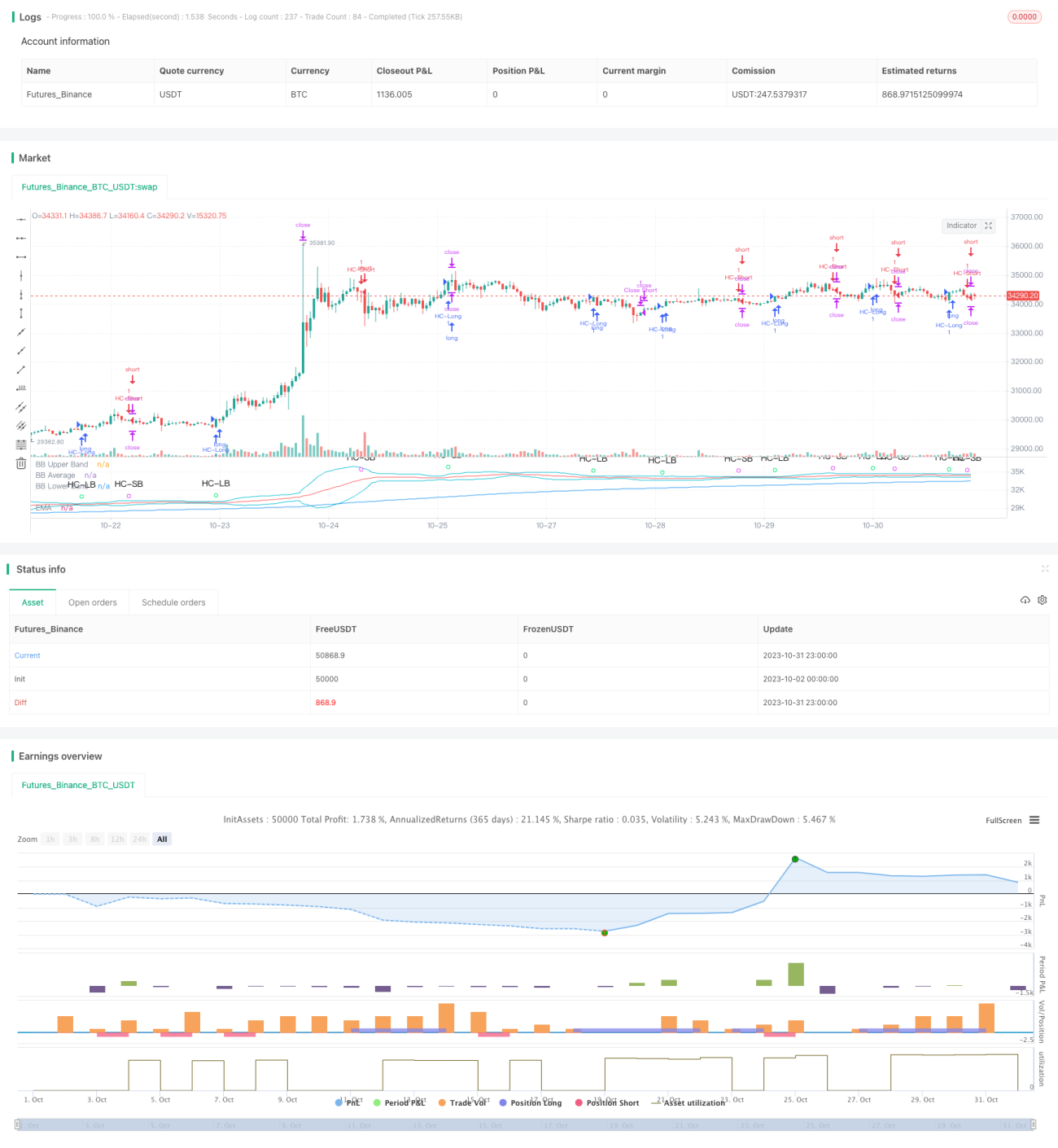
/*backtest
start: 2023-10-02 00:00:00
end: 2023-11-01 00:00:00
period: 1h
basePeriod: 15m
exchanges: [{"eid":"Futures_Binance","currency":"BTC_USDT"}]
*/

//@version=4

// This source code is subject to the terms of the Mozilla Public License 2.0 at https://mozilla.org/MPL/2.0/
// © MakeMoneyCoESTB2020- 1