Chiến lược phân kỳ rời rạc RSI


Ngày tạo: 2023-11-16 11:36:45 sửa đổi lần cuối: 2023-11-16 11:36:45
sao chép: 0 Số nhấp chuột: 862
1
tập trung vào
1617
Người theo dõi

Chiến lược phân kỳ rời rạc RSI

Tổng quan

Chiến lược này được đánh giá bởi các chỉ số RSI và đường trung bình EMA của nó để xác định tình huống giao thoa, và kết hợp RSI với giá để tìm kiếm điểm mua và bán tiềm năng. Chiến lược này thuộc về chiến lược theo dõi xu hướng.

Nguyên tắc chiến lược

  1. Chỉ số RSI có độ dài 14 được tính toán, khi RSI vượt qua đường phân chia 50 là tín hiệu xem nhiều và đi qua là tín hiệu nhìn xa.

  2. Tính toán đường trung bình 20 chu kỳ EMA và đường trung bình 14 chu kỳ EMA của RSI, khi đường nhanh đi qua đường chậm là tín hiệu mua, đường thấp đi qua là tín hiệu bán.

  3. Xác định sự lệch của RSI với giá:

  • Nhiều người quay lưng: Giá sáng tạo thấp nhưng RSI không sáng tạo thấp, tín hiệu mua

  • Giấu trộm đa đầu: Giá sáng tạo cao nhưng RSI không sáng tạo cao, tín hiệu mua

  • Giá sáng tạo cao nhưng RSI không sáng tạo cao, cho tín hiệu bán

  • Giấu tròn: Giá sáng tạo thấp nhưng RSI không sáng tạo thấp, cho tín hiệu bán

  1. Có thể chọn để kích hoạt chiến lược dừng lỗ, bao gồm dừng phần trăm và dừng ATR.

Phân tích lợi thế

  1. Ưu điểm của chỉ số RSI là có thể phát hiện tình trạng quá mua quá bán. Ưu điểm của đường trung bình EMA là có thể đóng vai trò làm mịn và làm giảm một phần tiếng ồn.

  2. RSI có thể đưa ra tín hiệu trước khi xu hướng đảo ngược.

  3. Tích hợp hai tín hiệu chỉ số có thể xác minh lẫn nhau, tăng sự ổn định của chiến lược.

  4. Cơ chế ngăn chặn thiệt hại có thể kiểm soát tổn thất đơn lẻ.

Phân tích rủi ro

  1. RSI là một chỉ số chỉ số biến động giá, khi giá biến động mạnh, hiệu quả của chỉ số RSI sẽ bị giảm giá.

  2. EMA cũng cho biết có một sự chậm trễ về thời gian, không thể xác định chính xác điểm chuyển hướng.

  3. Trong trường hợp biến động từ tín hiệu có thể xuất hiện tín hiệu giả, giá tiếp tục chạy theo xu hướng ban đầu.

  4. Thiết lập điểm dừng không hợp lý có thể gây ra tổn thất không cần thiết.

  5. Việc rút lui có thể lớn hơn và cần được hỗ trợ tài chính.

Hướng tối ưu hóa

  1. Bạn có thể thử nghiệm các tham số khác nhau để tính toán RSI và EMA, tìm kiếm sự kết hợp tốt nhất.

  2. Có thể xem xét thay thế đường trung bình EMA bằng các chỉ số khác như MACD để tối ưu hóa kết hợp.

  3. Có thể thiết lập cơ chế xác nhận để tránh sự lệch lạc giả. Nếu cần, nhiều tín hiệu lệch lạc liên tiếp sẽ được kích hoạt.

  4. Thêm chiến lược chặn để khóa lợi nhuận.

  5. Có thể tham gia dựa trên các tín hiệu ngắn hạn như mô hình nến và đánh giá xu hướng phù hợp với chiến lược này.

Tóm tắt

Chiến lược này tích hợp các phán đoán mua quá mức của chỉ số RSI, phán đoán xu hướng của EMA và dự đoán tín hiệu lệch hướng, tạo thành một hệ thống theo dõi xu hướng hoàn chỉnh hơn. Trên cơ sở điều chỉnh tham số và tối ưu hóa kết hợp, hiệu quả chiến lược tốt hơn có thể được đạt được. Tuy nhiên, vẫn cần chú ý để phòng ngừa các cú sốc của thị trường xu hướng và các tín hiệu sai lệch. Với quản lý vốn nghiêm ngặt, chiến lược này có thể đạt được lợi nhuận vượt trội ổn định trên đường dài trung bình.
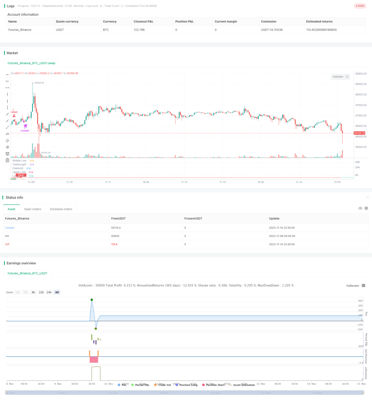
Mã nguồn chiến lược
/*backtest
start: 2023-11-08 00:00:00
end: 2023-11-15 00:00:00
period: 30m
basePeriod: 15m
exchanges: [{"eid":"Futures_Binance","currency":"BTC_USDT"}]
*/

//@version=4
strategy(title="RSI Divergence Indicator", overlay=false,pyramiding=2, default_qty_value=2,   default_qty_type=strategy.fixed, initial_capital=10000, currency=currency.USD)

len = input(title="RSI Period", minval=1, defval=14)
src = input(title="RSI Source", defval=close)
lbR = input(title="Pivot Lookback Right", defval=3)
lbL = input(title="Pivot Lookback Left", defval=1)
takeProfitRSILevel = input(title="Take Profit at RSI Level", minval=70, defval=80)

rangeUpper = input(title="Max of Lookback Range", defval=60)
rangeLower = input(title="Min of Lookback Range", defval=5)
plotBull = input(title="Plot Bullish", defval=true)
plotHiddenBull = input(title="Plot Hidden Bullish", defval=true)
plotBear = input(title="Plot Bearish", defval=true)
plotHiddenBear = input(title="Plot Hidden Bearish", defval=false)

sl_type = input("NONE", title="Trailing StopLoss Type", options=['ATR','PERC', 'NONE'])

stopLoss = input(title="Stop Loss%", defval=5, minval=1)

atrLength=input(14, title="ATR Length (for Trailing stop loss)")
atrMultiplier=input(3.5, title="ATR Multiplier (for Trailing stop loss)")


bearColor = color.red
bullColor = color.green
hiddenBullColor = color.new(color.green, 80)
hiddenBearColor = color.new(color.red, 80)
textColor = color.white
noneColor = color.new(color.white, 100)

osc = rsi(src, len)

plot(osc, title="RSI", linewidth=2, color=color.white)
hline(50, title="Middle Line", linestyle=hline.style_dotted)
obLevel = hline(70, title="Overbought", linestyle=hline.style_dotted)
osLevel = hline(30, title="Oversold", linestyle=hline.style_dotted)
fill(obLevel, osLevel, title="Background", color=color.gray, transp=90)

plFound = na(pivotlow(osc, lbL, lbR)) ? false : true
phFound = na(pivothigh(osc, lbL, lbR)) ? false : true

_inRange(cond) =>
    bars = barssince(cond == true)
    rangeLower <= bars and bars <= rangeUpper

//------------------------------------------------------------------------------
// Regular Bullish

// Osc: Higher Low
oscHL = osc[lbR] > valuewhen(plFound, osc[lbR], 1) and _inRange(plFound[1])

// Price: Lower Low
priceLL = low[lbR] < valuewhen(plFound, low[lbR], 1)

bullCond = plotBull and priceLL and oscHL and plFound

plot(
	 plFound ? osc[lbR] : na,
	 offset=-lbR,
	 title="Regular Bullish",
	 linewidth=2,
	 color=(bullCond ? bullColor : noneColor),
	 transp=0
	 )


plotshape(
	 bullCond ? osc[lbR] : na,
	 offset=-lbR,
	 title="Regular Bullish Label",
	 text=" Bull ",
	 style=shape.labelup,
	 location=location.absolute,
	 color=bullColor,
	 textcolor=textColor,
	 transp=0
	 )

//------------------------------------------------------------------------------
// Hidden Bullish

// Osc: Lower Low
oscLL = osc[lbR] < valuewhen(plFound, osc[lbR], 1) and _inRange(plFound[1])

// Price: Higher Low
priceHL = low[lbR] > valuewhen(plFound, low[lbR], 1)

hiddenBullCond = plotHiddenBull and priceHL and oscLL and plFound

plot(
	 plFound ? osc[lbR] : na,
	 offset=-lbR,
	 title="Hidden Bullish",
	 linewidth=2,
	 color=(hiddenBullCond ? hiddenBullColor : noneColor),
	 transp=0
	 )

plotshape(
	 hiddenBullCond ? osc[lbR] : na,
	 offset=-lbR,
	 title="Hidden Bullish Label",
	 text=" H Bull ",
	 style=shape.labelup,
	 location=location.absolute,
	 color=bullColor,
	 textcolor=textColor,
	 transp=0
	 )

longCondition=bullCond or hiddenBullCond
//? osc[lbR] : na  
//hiddenBullCond
strategy.entry(id="RSIDivLE", long=true,  when=longCondition)


//Trailing StopLoss
////// Calculate trailing SL
/////////////////////////////////////////////////////
sl_val = sl_type == "ATR"      ? stopLoss * atr(atrLength) : 
         sl_type == "PERC" ? close * stopLoss / 100 : 0.00

trailing_sl = 0.0
trailing_sl :=   strategy.position_size>=1 ?  max(low  - sl_val, nz(trailing_sl[1])) :  na

//draw initil stop loss
//plot(strategy.position_size>=1 ? trailing_sl : na, color = color.blue , style=plot.style_linebr,  linewidth = 2, title = "stop loss")
//plot(trailing_sl, title="ATR Trailing Stop Loss", style=plot.style_linebr, linewidth=1, color=color.purple, transp=30)
//Trailing StopLoss
////// Calculate trailing SL
/////////////////////////////////////////////////////


//------------------------------------------------------------------------------
// Regular Bearish

// Osc: Lower High
oscLH = osc[lbR] < valuewhen(phFound, osc[lbR], 1) and _inRange(phFound[1])

// Price: Higher High
priceHH = high[lbR] > valuewhen(phFound, high[lbR], 1)

bearCond = plotBear and priceHH and oscLH and phFound

plot(
	 phFound ? osc[lbR] : na,
	 offset=-lbR,
	 title="Regular Bearish",
	 linewidth=2,
	 color=(bearCond ? bearColor : noneColor),
	 transp=0
	 )

plotshape(
	 bearCond ? osc[lbR] : na,
	 offset=-lbR,
	 title="Regular Bearish Label",
	 text=" Bear ",
	 style=shape.labeldown,
	 location=location.absolute,
	 color=bearColor,
	 textcolor=textColor,
	 transp=0
	 )

//------------------------------------------------------------------------------
// Hidden Bearish

// Osc: Higher High
oscHH = osc[lbR] > valuewhen(phFound, osc[lbR], 1) and _inRange(phFound[1])

// Price: Lower High
priceLH = high[lbR] < valuewhen(phFound, high[lbR], 1)

hiddenBearCond = plotHiddenBear and priceLH and oscHH and phFound

plot(
	 phFound ? osc[lbR] : na,
	 offset=-lbR,
	 title="Hidden Bearish",
	 linewidth=2,
	 color=(hiddenBearCond ? hiddenBearColor : noneColor),
	 transp=0
	 )

plotshape(
	 hiddenBearCond ? osc[lbR] : na,
	 offset=-lbR,
	 title="Hidden Bearish Label",
	 text=" H Bear ",
	 style=shape.labeldown,
	 location=location.absolute,
	 color=bearColor,
	 textcolor=textColor,
	 transp=0
	 )
longCloseCondition=crossover(osc,takeProfitRSILevel) or bearCond
strategy.close(id="RSIDivLE", comment="Close All="+tostring(close - strategy.position_avg_price, "####.##"), when= abs(strategy.position_size)>=1  and  sl_type == "NONE" and longCloseCondition)

//close all on stop loss
strategy.close(id="RSIDivLE", comment="TSL="+tostring(close - strategy.position_avg_price, "####.##"),  when=abs(strategy.position_size)>=1 and (sl_type == "PERC"   or sl_type == "ATR" ) and crossunder(close, trailing_sl)  )  //close<ema55 and rsi5Val<20 //ema34<ema55  //close<ema89

src1 = close, 
len6 = input(14, minval=1, title="RSI Length")
len7 = input(20, minval=1, title="EMA of RSI Length")
len8 = input(14,minval=1, title="Fast EMA")
up = rma(max(change(src1), 0), len6)
down = rma(-min(change(src1), 0), len6)
rsi = down == 0 ? 100 : up == 0 ? 0 : 100 - (100 / (1 + up / down))
emaRSI = ema(rsi,len7)
fastEmaRSI=ema(rsi,len8)

plot(emaRSI, title="EMA of RSI", linewidth=1, color=color.red)
plot(fastEmaRSI,title="Fast EMA of RSI", linewidth=1,color = color.lime)
band1 = hline(80, title="Upper Line", linewidth=1, color=color.red)
band0 = hline(20, title="Lower Line", linewidth=1, color=color.lime)
fill(band1, band0, color=color.purple)