BEAM ব্যান্ডের উপর ভিত্তি করে BTCdollar খরচ গড় কৌশল

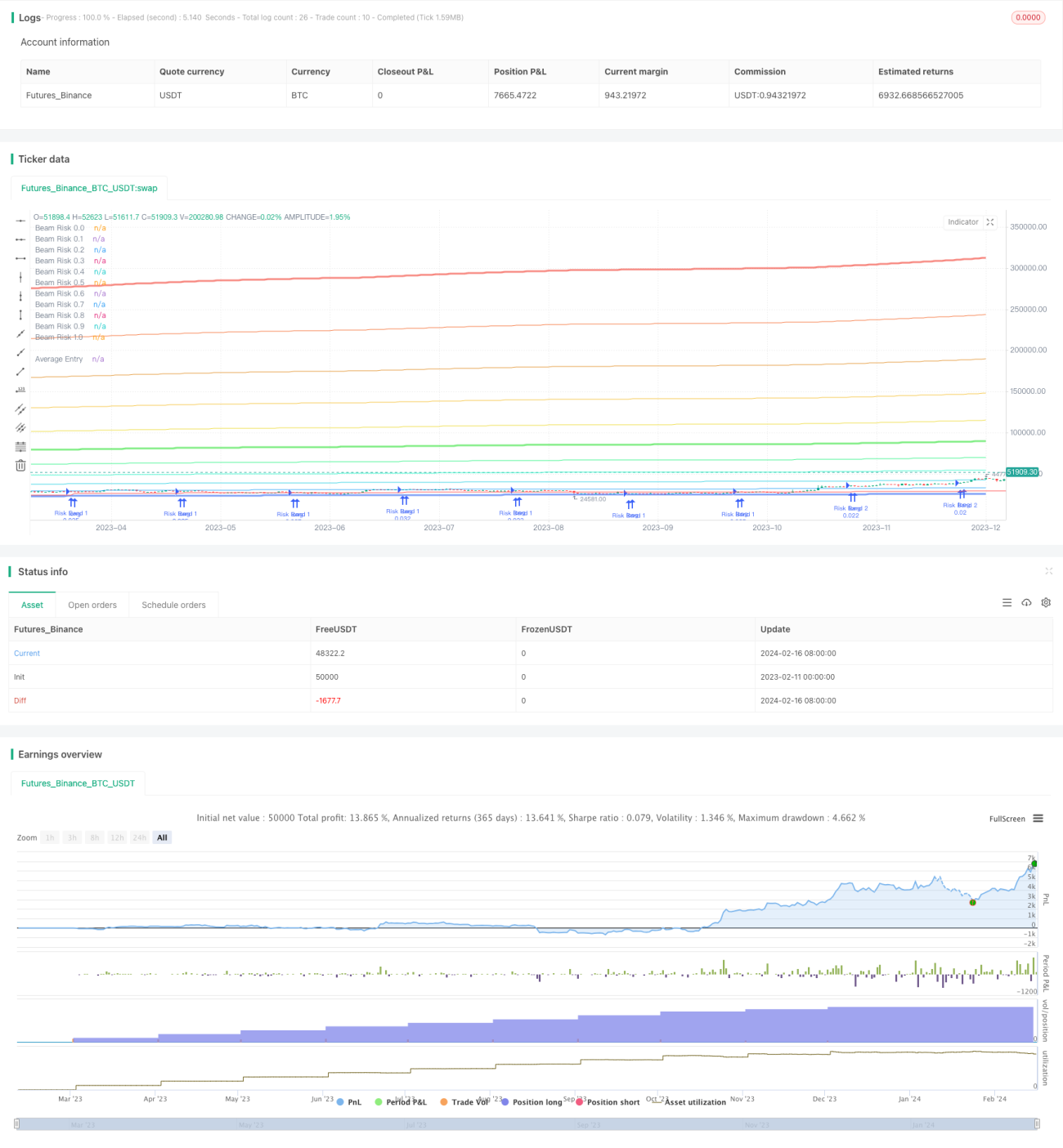
/*backtest
start: 2023-02-11 00:00:00
end: 2024-02-17 00:00:00
period: 1d
basePeriod: 1h
exchanges: [{"eid":"Futures_Binance","currency":"BTC_USDT"}]
*/

// © gjfsdrtytru - BEAM DCA Strategy {
// Based on Ben Cowen's risk level strategy, this aims to copy that method but with BEAM band levels.
// Upper BEAM level is derived from ln(price/200W MA)/2.5, while the 200W MA is the floor price. This is our 0-1 range. 
// Buy limit orders are set at the < 0.5 levels and sell orders are set at the > 0.5 level.
//@version=5
strategy(
  title                 = "BEAM DCA Strategy Monthly", 
  shorttitle            = "BEAM DCA M",
  overlay               = true,
  pyramiding            = 500,
  default_qty_type      = strategy.percent_of_equity,
  default_qty_value     = 0,
  initial_capital       = 0) //}

// Inputs { ————————————————————————————————————————————————————————————————————
T_ceiling   = input.string("Off", "Diminishing Returns", ["Off","Linear","Parabolic"], "Account for diminishing returns as time increases")
day         = input.int(1, "DCA Day of Month",1,28,1,"Select day of month for buy orders.")
DCAamount   = input.int(1000,"DCA Amount",400,tooltip="Enter the maximum amount you'd be willing to DCA for any given month.")
T_buy       = input(true,"Buy Orders","Toggle buy orders.")
T_sell      = input(true,"Sell Orders","Toggle sell orders.")

// Time period
testStartYear   = input.int(2018,   title="Backtest Start Year",    minval=2010,maxval=2100,group="Backtest Period")
testStartMonth  = input.int(1,      title="Backtest Start Month",   minval=1,   maxval=12,  group="Backtest Period")
testStartDay    = input.int(1,      title="Backtest Start Day",     minval=1,   maxval=31,  group="Backtest Period")
testPeriodLen   = input.int(9999,   title="Backtest Period (days)", minval=1,               group="Backtest Period",tooltip="Days until strategy ends") * 86400000 // convert days into UNIX time
testPeriodStart = timestamp(testStartYear,testStartMonth,testStartDay,0,0)
testPeriodStop  = testPeriodStart + testPeriodLen
testPeriod() => true
// ——————————————————————————————————————————————————————————————————————————— }
// Diminishing Returns { ———————————————————————————————————————————————————————
x = bar_index + 1
assetDivisor= 2.5
switch
    T_ceiling == "Linear"   => assetDivisor:= 3.50542 - 0.000277696 * x
    T_ceiling == "Parabolic"=> assetDivisor:= -0.0000001058992338 * math.pow(x,2) + 0.000120729 * x + 3.1982
// ——————————————————————————————————————————————————————————————————————————— }
// Risk Levels { ———————————————————————————————————————————————————————————————
cycleLen = 1400
getMaLen() =>
    if bar_index < cycleLen
        bar_index + 1
    else
        cycleLen

// Define Risk Bands
price       = close
riskLow     = ta.sma(price,getMaLen())
risk1       = riskLow * math.exp((assetDivisor)*0.1)
risk2       = riskLow * math.exp((assetDivisor)*0.2)
risk3       = riskLow * math.exp((assetDivisor)*0.3)
risk4       = riskLow * math.exp((assetDivisor)*0.4)
risk5       = riskLow * math.exp((assetDivisor)*0.5)
risk6       = riskLow * math.exp((assetDivisor)*0.6)
risk7       = riskLow * math.exp((assetDivisor)*0.7)
risk8       = riskLow * math.exp((assetDivisor)*0.8)
risk9       = riskLow * math.exp((assetDivisor)*0.9)
riskHigh    = riskLow * math.exp((assetDivisor))

// Plot Risk Bands
p_low       = plot(riskLow,   "Beam Risk 0.0",color.new(#0042F0,50),3,editable=false)
p_band1     = plot(risk1,     "Beam Risk 0.1",color.new(#0090F5,20),1,editable=false)
p_band2     = plot(risk2,     "Beam Risk 0.2",color.new(#00C6DB,20),1,editable=false)
p_band3     = plot(risk3,     "Beam Risk 0.3",color.new(#00F5BD,20),1,editable=false)
p_band4     = plot(risk4,     "Beam Risk 0.4",color.new(#00F069,20),1,editable=false)
p_band5     = plot(risk5,     "Beam Risk 0.5",color.new(#00DB08,50),3,editable=false)
p_band6     = plot(risk6,     "Beam Risk 0.6",color.new(#E8D20C,20),1,editable=false)
p_band7     = plot(risk7,     "Beam Risk 0.7",color.new(#F2B40C,20),1,editable=false)
p_band8     = plot(risk8,     "Beam Risk 0.8",color.new(#DC7A00,20),1,editable=false)
p_band9     = plot(risk9,     "Beam Risk 0.9",color.new(#F2520C,20),1,editable=false)
p_band10    = plot(riskHigh,  "Beam Risk 1.0",color.new(#F01102,50),3,editable=false)
// ——————————————————————————————————————————————————————————————————————————— }
// Order Execution { ———————————————————————————————————————————————————————————
band5   = price<risk5 and price>risk4
band4   = price<risk4 and price>risk3
band3   = price<risk3 and price>risk2
band2   = price<risk2 and price>risk1
band1   = price<risk1

// DCA buy order weights
y       = DCAamount / 5
switch
    band5 => y:= y * 1
    band4 => y:= y * 2
    band3 => y:= y * 3
    band2 => y:= y * 4
    band1 => y:= y * 5

// Contracts per order
contracts =(y/price)

if testPeriod()
// Buy orders
    if T_buy == true
        if dayofmonth == day
            strategy.entry("Risk Band 5",strategy.long,qty=contracts,when=band5)
            strategy.entry("Risk Band 4",strategy.long,qty=contracts,when=band4)
            strategy.entry("Risk Band 3",strategy.long,qty=contracts,when=band3)
            strategy.entry("Risk Band 2",strategy.long,qty=contracts,when=band2)
            strategy.entry("Risk Band 1",strategy.long,qty=contracts,when=band1)
// Sell orders 
    if T_sell == true
        if strategy.opentrades > 5
            strategy.exit("Risk Band 6",qty_percent=6.67,limit=risk6) 
            strategy.exit("Risk Band 7",qty_percent=14.28,limit=risk7)
            strategy.exit("Risk Band 8",qty_percent=25.00,limit=risk8)
            strategy.exit("Risk Band 9",qty_percent=44.44,limit=risk9)
            strategy.exit("Risk Band 10",qty_percent=100,limit=riskHigh)
// ——————————————————————————————————————————————————————————————————————————— }
// Info { ——————————————————————————————————————————————————————————————————————

// Line plot of avg. entry price
plot(strategy.position_size > 0 ? strategy.position_avg_price : na,"Average Entry",color.red,trackprice=true,editable=false)

// Unrealised PNL
uPNL = price/strategy.position_avg_price

// Realised PNL
realPNL = 0.
for i = 0 to strategy.closedtrades-1
    realPNL += strategy.closedtrades.profit(i)

// Size of open position in ($)
openPosSize = 0.
for i = 0 to strategy.opentrades-1
    openPosSize += strategy.opentrades.size(i) * strategy.position_avg_price

// Size of closed position in ($)
closePosSize = 0.
if strategy.closedtrades > 0
    for i = 0 to strategy.closedtrades-1
        closePosSize += strategy.closedtrades.size(i) * strategy.closedtrades.entry_price(i)

invested    = openPosSize+closePosSize                              // Total capital ($) put into strategy
equity      = openPosSize+closePosSize+strategy.openprofit+realPNL  // Total current equity ($) in strategy (counting realised PNL)
ROI         = (equity-invested) / invested * 100                    // ROI of strategy (compare capital invested to excess return)

// // Info Table
// var table table1 = table.new(position.bottom_right,2,9,color.black,color.gray,1,color.gray,2)

// table.cell(table1,0,0,"Capital Invested",   text_color=color.white,text_halign=text.align_right)
// table.cell(table1,0,1,"Open Position",      text_color=color.white,text_halign=text.align_right)
// table.cell(table1,0,2,"Average Entry",      text_color=color.white,text_halign=text.align_right)
// table.cell(table1,0,3,"Last Price",         text_color=color.white,text_halign=text.align_right)
// table.cell(table1,0,4,"Open PNL (%)",       text_color=color.white,text_halign=text.align_right)
// table.cell(table1,0,5,"Open PNL ($)",       text_color=color.white,text_halign=text.align_right)
// table.cell(table1,0,6,"Realised PNL ($)",   text_color=color.white,text_halign=text.align_right)
// table.cell(table1,0,7,"Total Equity",       text_color=color.white,text_halign=text.align_right)
// table.cell(table1,0,8,"Strategy ROI",       text_color=color.white,text_halign=text.align_right)

// table.cell(table1,1,0,"$" + str.tostring(invested,                      "#,###.00"),      text_halign=text.align_right,text_color = color.white)
// table.cell(table1,1,1,"$" + str.tostring(openPosSize,                   "#,###.00"),      text_halign=text.align_right,text_color = color.white)
// table.cell(table1,1,2,"$" + str.tostring(strategy.position_avg_price,   "#,###.00"),      text_halign=text.align_right,text_color = color.white)
// table.cell(table1,1,3,"$" + str.tostring(price,                         "#,###.00"),      text_halign=text.align_right,text_color = color.white)
// table.cell(table1,1,4,      str.tostring((uPNL-1)*100,                  "#,###.00") + "%",text_halign=text.align_right,text_color = uPNL > 1 ? color.lime : color.red)
// table.cell(table1,1,5,"$" + str.tostring(strategy.openprofit,           "#,###.00"),      text_halign=text.align_right,text_color = uPNL > 1 ? color.lime : color.red)
// table.cell(table1,1,6,"$" + str.tostring(realPNL,                       "#,###.00"),      text_halign=text.align_right,text_color = color.white)
// table.cell(table1,1,7,"$" + str.tostring(equity,                        "#,###.00"),      text_halign=text.align_right,text_color = color.white)
// table.cell(table1,1,8,      str.tostring(ROI,                           "#,###.00") + "%",text_halign=text.align_right,text_color = ROI > 1 ? color.lime : color.red)
// // ——————————————————————————————————————————————————————————————————————————— }