Esta estrategia es una estrategia bidireccional de seguimiento de impulso de filtro de rango adaptativo

El autor:¿ Qué pasa?, Fecha: 2024-01-24 11:31:51
Las etiquetas:

Resumen general

Esta estrategia es una estrategia bidireccional de seguimiento de impulso de filtro de rango adaptativo. Utiliza un filtro de rango adaptativo para rastrear las fluctuaciones de precios y combina indicadores de volumen para determinar la dirección del valor, con el fin de implementar compras bajas y ventas altas.

Principios de estrategia

Utilice un filtro de rango adaptativo para rastrear las fluctuaciones de precios.
Hay dos tipos de filtros: Tipo 1 y Tipo 2.
Determine la dirección de la fluctuación de los precios basándose en la relación entre el filtro y el precio de cierre.
Combinado con el aumento y la caída del precio de cierre en comparación con el día anterior, determina la dirección del valor.
Emitir una señal de compra cuando el precio rompe la pista superior y el valor aumenta; Emitir una señal de venta cuando el precio rompe la pista inferior y el valor cae.

Análisis de ventajas

El filtro de rango adaptativo puede capturar con precisión las fluctuaciones del mercado.
Dos tipos de filtros pueden satisfacer diferentes preferencias comerciales.
La combinación de indicadores de volumen puede identificar eficazmente la dirección del valor.
La estrategia es flexible y los parámetros pueden ajustarse según las condiciones del mercado.
Lógico de condiciones comerciales personalizable.

Análisis de riesgos

La configuración incorrecta de los parámetros puede dar lugar a un exceso de operaciones o a operaciones perdidas.
Las señales de fuga tienen cierto retraso.
Los indicadores de volumen tienen cierto riesgo de estancamiento.
Las rupturas de alcance son propensas a quedar atrapadas.

Prevención de riesgos:

Elegir las combinaciones de parámetros adecuadas y ajustarlas oportunamente.
Combinar otros indicadores para identificar las tendencias.
Comerciar con cautela alrededor de los niveles clave y inversiones de tendencia.

Direcciones de optimización

Prueba diferentes combinaciones de tamaños de rango y ciclos de suavizado para encontrar la combinación óptima.
Prueba diferentes tipos de filtros y elige el tipo que prefieras.
Experimentación con otros indicadores de volumen o indicadores técnicos auxiliares.
Optimizar y ajustar la lógica de las condiciones de negociación para reducir el comercio irracional.
Incorporar teoremas de mercado para establecer el tamaño de posición adaptativo.

/*backtest
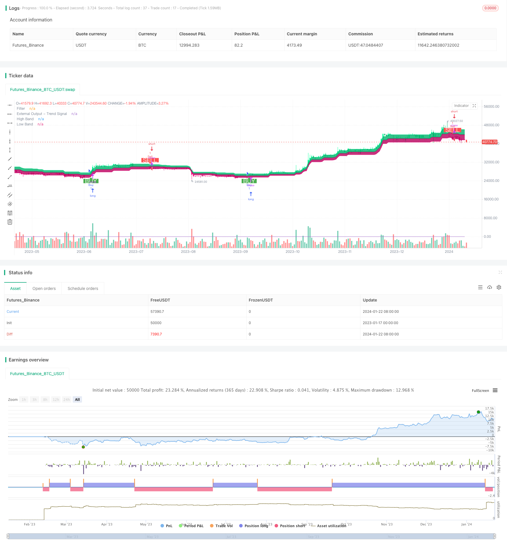
start: 2023-01-17 00:00:00
end: 2024-01-23 00:00:00
period: 1d
basePeriod: 1h
exchanges: [{"eid":"Futures_Binance","currency":"BTC_USDT"}]
*/

//@version=4
strategy("Range Filter [DW] & Labels", shorttitle="RF [DW] & Labels", overlay=true)


//Conditional Sampling EMA Function 
Cond_EMA(x, cond, n)=>
    var val     = array.new_float(0)
    var ema_val = array.new_float(1)
    if cond
        array.push(val, x)
        if array.size(val) > 1
            array.remove(val, 0)
        if na(array.get(ema_val, 0))
            array.fill(ema_val, array.get(val, 0))
        array.set(ema_val, 0, (array.get(val, 0) - array.get(ema_val, 0))*(2/(n + 1)) + array.get(ema_val, 0))
    EMA = array.get(ema_val, 0)
    EMA

//Conditional Sampling SMA Function
Cond_SMA(x, cond, n)=>
    var vals = array.new_float(0)
    if cond
        array.push(vals, x)
        if array.size(vals) > n
            array.remove(vals, 0)
    SMA = array.avg(vals)
    SMA

//Standard Deviation Function
Stdev(x, n)=>
    sqrt(Cond_SMA(pow(x, 2), 1, n) - pow(Cond_SMA(x, 1, n), 2))

//Range Size Function
rng_size(x, scale, qty, n)=> 
    ATR      = Cond_EMA(tr(true), 1, n)
    AC       = Cond_EMA(abs(x - x[1]), 1, n)
    SD       = Stdev(x, n)
    rng_size = scale=="Pips" ? qty*0.0001 : scale=="Points" ? qty*syminfo.pointvalue : scale=="% of Price" ? close*qty/100 : scale=="ATR" ? qty*ATR :
               scale=="Average Change" ? qty*AC : scale=="Standard Deviation" ? qty*SD : scale=="Ticks" ? qty*syminfo.mintick : qty   

//Two Type Range Filter Function
rng_filt(h, l, rng_, n, type, smooth, sn, av_rf, av_n)=>
    rng_smooth = Cond_EMA(rng_, 1, sn)
    r          = smooth ? rng_smooth : rng_
    var rfilt  = array.new_float(2, (h + l)/2)
    array.set(rfilt, 1, array.get(rfilt, 0))
    if type=="Type 1"
        if h - r > array.get(rfilt, 1)
            array.set(rfilt, 0, h - r)
        if l + r < array.get(rfilt, 1)
            array.set(rfilt, 0, l + r)
    if type=="Type 2"
        if h >= array.get(rfilt, 1) + r
            array.set(rfilt, 0, array.get(rfilt, 1) + floor(abs(h - array.get(rfilt, 1))/r)*r)
        if l <= array.get(rfilt, 1) - r
            array.set(rfilt, 0, array.get(rfilt, 1) - floor(abs(l - array.get(rfilt, 1))/r)*r)
    rng_filt1 = array.get(rfilt, 0)
    hi_band1  = rng_filt1 + r
    lo_band1  = rng_filt1 - r
    rng_filt2 = Cond_EMA(rng_filt1, rng_filt1 != rng_filt1[1], av_n)
    hi_band2  = Cond_EMA(hi_band1, rng_filt1 != rng_filt1[1], av_n)
    lo_band2  = Cond_EMA(lo_band1, rng_filt1 != rng_filt1[1], av_n)
    rng_filt  = av_rf ? rng_filt2 : rng_filt1
    hi_band   = av_rf ? hi_band2 : hi_band1
    lo_band   = av_rf ? lo_band2 : lo_band1
    [hi_band, lo_band, rng_filt]
 
//-----------------------------------------------------------------------------------------------------------------------------------------------------------------
//Inputs
//-----------------------------------------------------------------------------------------------------------------------------------------------------------------

//Filter Type
f_type = input(defval="Type 1", options=["Type 1", "Type 2"], title="Filter Type")

//Movement Source
mov_src = input(defval="Close", options=["Wicks", "Close"], title="Movement Source")

//Range Size Inputs
rng_qty   = input(defval=2.618, minval=0.0000001, title="Range Size")
rng_scale = input(defval="Average Change", options=["Points", "Pips", "Ticks", "% of Price", "ATR", "Average Change", "Standard Deviation", "Absolute"], title="Range Scale")

//Range Period
rng_per = input(defval=14, minval=1, title="Range Period (for ATR, Average Change, and Standard Deviation)")

//Range Smoothing Inputs
smooth_range = input(defval=true, title="Smooth Range")
smooth_per   = input(defval=27, minval=1, title="Smoothing Period")

//Filter Value Averaging Inputs
av_vals    = input(defval=true, title="Average Filter Changes")
av_samples = input(defval=2, minval=1, title="Number Of Changes To Average")

//-----------------------------------------------------------------------------------------------------------------------------------------------------------------
//Definitions
//-----------------------------------------------------------------------------------------------------------------------------------------------------------------

//High And Low Values
h_val = mov_src=="Wicks" ? high : close
l_val = mov_src=="Wicks" ? low : close

//Range Filter Values
[h_band, l_band, filt] = rng_filt(h_val, l_val, rng_size((h_val + l_val)/2, rng_scale, rng_qty, rng_per), rng_per, f_type, smooth_range, smooth_per, av_vals, av_samples)

//Direction Conditions
var fdir = 0.0
fdir    := filt > filt[1] ? 1 : filt < filt[1] ? -1 : fdir
upward   = fdir==1 ? 1 : 0
downward = fdir==-1 ? 1 : 0

//Colors
filt_color = upward ? #05ff9b : downward ? #ff0583 : #cccccc
bar_color  = upward and (close > filt) ? (close > close[1] ? #05ff9b : #00b36b) :
             downward and (close < filt) ? (close < close[1] ? #ff0583 : #b8005d) : #cccccc

//-----------------------------------------------------------------------------------------------------------------------------------------------------------------
//Outputs
//-----------------------------------------------------------------------------------------------------------------------------------------------------------------

//Filter Plot
filt_plot = plot(filt, color=filt_color, transp=0, linewidth=3,  title="Filter")

//Band Plots
h_band_plot = plot(h_band, color=#05ff9b, transp=100, title="High Band")
l_band_plot = plot(l_band, color=#ff0583, transp=100, title="Low Band")

//Band Fills
fill(h_band_plot, filt_plot, color=#00b36b, transp=85, title="High Band Fill")
fill(l_band_plot, filt_plot, color=#b8005d, transp=85, title="Low Band Fill")

//Bar Color
barcolor(bar_color)

//External Trend Output
plot(fdir, transp=100, editable=false, display=display.none, title="External Output - Trend Signal")

// Trading Conditions Logic
longCond = close > filt and close > close[1] and upward > 0 or close > filt and close < close[1] and upward > 0 
shortCond = close < filt and close < close[1] and downward > 0 or close < filt and close > close[1] and downward > 0

CondIni = 0
CondIni := longCond ? 1 : shortCond ? -1 : CondIni[1]
longCondition = longCond and CondIni[1] == -1
shortCondition = shortCond and CondIni[1] == 1

// Strategy Entry and Exit
strategy.entry("Buy", strategy.long, when = longCondition)
strategy.entry("Sell", strategy.short, when = shortCondition)

strategy.close("Buy", when = shortCondition)
strategy.close("Sell", when = longCondition)

// Plot Buy and Sell Labels
plotshape(longCondition, title = "Buy Signal", text ="BUY", textcolor = color.white, style=shape.labelup, size = size.normal, location=location.belowbar, color = color.green, transp = 0)
plotshape(shortCondition, title = "Sell Signal", text ="SELL", textcolor = color.white, style=shape.labeldown, size = size.normal, location=location.abovebar, color = color.red, transp = 0)

// Alerts
alertcondition(longCondition, title="Buy Alert", message = "BUY")
alertcondition(shortCondition, title="Sell Alert", message = "SELL")

Más.