Estrategia de cazador de tendencias de marcos temporales múltiples


Fecha de creación: 2024-02-18 10:17:06 Última modificación: 2024-02-18 10:17:06
Copiar: 0 Número de Visitas: 681
1
Seguir
1617
Seguidores

Estrategia de cazador de tendencias de marcos temporales múltiples

Descripción general

La estrategia de caza de tendencias de marco temporal múltiple es una estrategia que utiliza varios indicadores en combinación con señales de negociación automatizadas. La estrategia combina el uso de promedios móviles, indicadores de tendencias súper y indicadores de gráficos en una nube para juzgar la dirección de la tendencia en varios marcos de tiempo para descubrir oportunidades potenciales de negociación.

Principio de estrategia

El principio central de la estrategia es determinar la dirección de la tendencia en el marco de tiempo alto y en el marco de tiempo bajo al mismo tiempo. La estrategia primero calcula los promedios móviles clave, las líneas de tendencia súper y las líneas de conversión, las líneas de referencia, etc., en el marco de tiempo alto. Luego calcula las líneas de tendencia súper en el marco de tiempo bajo.

Una vez que se cumplen ciertas condiciones, la estrategia genera una señal de compra o venta. El usuario puede elegir si desea negociar solo una, una o ambas opciones según sus necesidades. Además, el usuario puede configurar parámetros de promedio móvil, parámetros de tendencia súper, parámetros de gráfico en una nube, etc., para optimizar el rendimiento de la estrategia.

Análisis de las ventajas

La mayor ventaja de esta estrategia reside en la combinación de múltiples marcos de tiempo y múltiples indicadores, lo que puede mejorar considerablemente la precisión de la dirección de la tendencia y detectar oportunamente oportunidades de reversión. Las ventajas concretas son:

  1. Aproveche los marcos de tiempo para confirmar tendencias y evitar ser engañado por el ruido del mercado
  2. Las medias móviles como indicadores de línea media y larga para determinar la dirección de las principales tendencias
  3. Las líneas de tendencia súper como indicadores a corto plazo para capturar el cambio de tendencia a tiempo
  4. Un mapa de la nube para determinar las áreas de resistencia y encontrar oportunidades potenciales

Análisis de riesgos

El principal riesgo de esta estrategia reside en que la configuración incorrecta de los parámetros puede conducir a operaciones demasiado frecuentes o oportunidades perdidas. Además, los indicadores que emiten señales erróneas también pueden causar pérdidas. Los riesgos específicos y las soluciones son los siguientes:

  1. Riesgo de configuración de parámetros: realizar más pruebas y optimización para encontrar la combinación óptima de parámetros
  2. Riesgo de error de señal: combinar más indicadores para verificar y evitar errores de señal
  3. Riesgo de retirada: ajuste adecuado de la gestión de las posiciones, control de las pérdidas individuales

Dirección de optimización

La estrategia tiene espacio para ser optimizada aún más:

  1. Añadir más combinaciones de indicadores, como las bandas de Brin, RSI, etc., para mejorar la precisión de los juicios
  2. Modelos integrados de aprendizaje automático para estrategias de negociación más inteligentes
  3. Combinación de tecnologías cuantitativas, como el comercio de alta frecuencia, los pájaros tempranos, para mejorar aún más el rendimiento de la estrategia
  4. Optimizar las estrategias de gestión de posiciones para reducir el riesgo de retiro mediante el ajuste dinámico de posiciones

Resumir

En resumen, la estrategia de caza de tendencias de múltiples marcos temporales utiliza múltiples indicadores y marcos temporales para determinar las tendencias y aprovechar oportunamente las oportunidades de reversión, es una estrategia de comercio cuantitativa de buen rendimiento. La estrategia tiene una alta integración y una amplia aplicación, y en el futuro todavía hay un gran espacio de optimización, que vale la pena que los comerciantes cuantitativos sigan estudiando y aplicando.
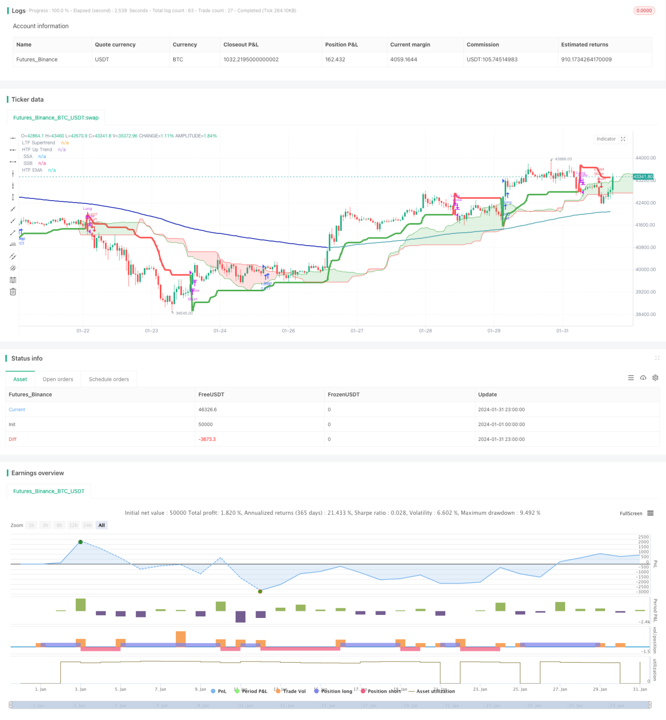
Código Fuente de la Estrategia
/*backtest
start: 2024-01-01 00:00:00
end: 2024-01-31 23:59:59
period: 1h
basePeriod: 15m
exchanges: [{"eid":"Futures_Binance","currency":"BTC_USDT"}]
*/

// This Pine Script™ code is subject to the terms of the Mozilla Public License 2.0 at https://mozilla.org/MPL/2.0/
// © godzcopilot / blockybears

// Thanks to anthonyf50 for his MTF Ichimoku https://www.tradingview.com/script/Pw9cBFma/
// Thanks to KivancOzbilgic for his SuperTrend https://www.tradingview.com/script/r6dAP7yi/
// Thanks to ZenAndTheArtOfTrading / PineScriptMastery for their Higher Timeframe EMA https://www.tradingview.com/script/Vh3XG9sD-Higher-Timeframe-EMA/


//@version=5
strategy("TrendHunter [Blocky]", overlay=true, default_qty_type=strategy.percent_of_equity, default_qty_value=80, initial_capital=1000, pyramiding=0)

// ================
// Strategy Inputs
// ================

// Defines user inputs for configuring the strategy.

// Higher Time Frame Selection
HTF_TimeFrame = input.timeframe(title='Higher Time Frame', defval='60', group = '== Timeframe ==', tooltip = "Select Chart for standard functionality")

// Inputs for EMA
len     = input.int(title="EMA Length", defval=200, group ='== EMA ==')
col     = input.bool(title="Colour EMA", defval=true, group ='== EMA ==')

// SuperTrend
Periods = input(title='ATR Period', defval=10, group = '== Supertrend ==')
Multiplier = input.float(title='ATR Multiplier', step=0.1, defval=3.0, group = '== Supertrend ==')
Src = input.source(title='Source', defval=hl2, group = '== Supertrend ==')

// Ichimoku
conversionPeriods = input.int(9, minval=1, title='Conversion Line Periods', group = '== Ichimoku ==')
basePeriods = input.int(26, minval=1, title='Base Line Periods', group = '== Ichimoku ==')
laggingSpan2Periods = input.int(52, minval=1, title='Lagging Span 2 Periods', group = '== Ichimoku ==')
displacement = input.int(26, minval=1, title='Displacement', group = '== Ichimoku ==')

// Ichimoku Display Options
isActiveConversion = input(false, 'Conversion Line', group = '== Ichimoku ==', inline = 'lines1')
isActiveBase = input(false, 'Base Line', group = '== Ichimoku ==', inline = 'lines1')
isActiveLagging = input(false, 'Lagging Span', group = '== Ichimoku ==', inline = 'lines2')
isActiveCloud = input(true, 'Cloud', group = '== Ichimoku ==', inline = 'lines2')


// ================
// Strategy Options
// ================

bTable = input.bool(true, title='Trade Table', group='== Strategy Options ==', tooltip = "Show table that shows current selected options and trade trade entry parameters")

bLong = input.bool(true, title='Enter Longs', group='== Strategy Options ==', inline = 'LongShort')
bShort = input.bool(true, title='Enter Shorts', group='== Strategy Options ==', inline = 'LongShort', tooltip = "Filter long / short trade signals")

bPriceCloud = input.bool(true, title='Price outside cloud', group='== Strategy Options ==', inline='PriceCloud')
bPriceCloudBody = input.bool(false, title='Full Body', group='== Strategy Options ==', inline='PriceCloud', tooltip = 'Only trade when price action outside the cloud.\nLongs when price action above the cloud.\nShort when price action below the cloud')

bPriceEMA = input.bool(false, title='Price above/below EMA', group='== Strategy Options ==', inline='PriceEMA')
bPriceEMABody = input.bool(false, title='Full Body', group='== Strategy Options ==', inline='PriceEMA', tooltip = 'Longs when price action above the EMA.\nShort when price action below the EMA')

bSuper = input.bool(true, title='Supertrend transistions', group='== Strategy Options ==', tooltip = "Trade in direction of the supertrend transitions")
bLTF = input.bool(false, title='LTF/HTF Supertrend alignment', group='== Strategy Options ==', tooltip = "Utilise a dual supertrends, chart and defined higher time frame")

bEMACloud1 = input.bool(true, title='EMA Outside Cloud', group='== Strategy Options ==', tooltip = "EMA must be outside the ichimoku cloud")
bEMACloud2 = input.bool(false, title='EMA above/below Cloud', group='== Strategy Options ==', tooltip = "Longs when EMA above the cloud.\nShort when EMA below the cloud")

bExitHTFTrail = input.bool(true, title='Super Trend Exits:  HTF', group='== Strategy Options ==', inline = 'Exits')
bExitLTFTrail = input.bool(true, title='LTF', group='== Strategy Options ==', inline = 'Exits', tooltip = 'Exit trades when price crosses the supertrend line\nIf neither selected trade closes when opposite trade opens\nIf using LTF closes turn on HTF/LTF alignment')

// ===========================
// EMA Functions and Plotting
// ===========================

// Calculate EMA
ema = ta.ema(close, len)
emaSmooth = request.security(syminfo.tickerid, HTF_TimeFrame, ema[barstate.isrealtime ? 1 : 0], gaps=barmerge.gaps_on)[barstate.isrealtime ? 0 : 1]


// Draw EMA
plot(emaSmooth, color=col ? (close > emaSmooth ? color.rgb(76, 163, 175) : color.rgb(6, 23, 173)) : color.black, linewidth=2, title="HTF EMA")


// ==================================
// Supertrend Functions and Plotting
// ==================================

// Function to calculate SuperTrend
calcSuperTrend(src, atrPeriods, multiplier) =>
    atr = ta.atr(atrPeriods)
    up = src - multiplier * atr
    up1 = nz(up[1], up)
    up := close[1] > up1 ? math.max(up, up1) : up
    dn = src + multiplier * atr
    dn1 = nz(dn[1], dn)
    dn := close[1] < dn1 ? math.min(dn, dn1) : dn
    trend = 1
    trend := nz(trend[1], trend)
    trend := trend == -1 and close > dn1 ? 1 : trend == 1 and close < up1 ? -1 : trend
    [up, dn, trend]

// Calculate SuperTrend for the current time frame
[up, dn, trend] = calcSuperTrend(Src, Periods, Multiplier)

// Plotting for the current time frame
plot(trend == 1 ? up : dn, title='LTF Supertrend', color=trend == 1 ?color.green : color.red, linewidth=1, style = plot.style_stepline)

// Fetching the higher time frame data
[HTF_up, HTF_dn, HTF_trend] = request.security(syminfo.tickerid, HTF_TimeFrame, calcSuperTrend(hl2, Periods, Multiplier), lookahead=barmerge.lookahead_on)

// Plotting for the higher time frame
plot(HTF_trend == 1 ? HTF_up : HTF_dn, title='HTF Up Trend', color= HTF_trend == 1 ? color.green : color.red, linewidth=4)


// ===============================
// Ichimoku Functions and Plotting
// ===============================

// Function to convert timeframe to hours
f_convertTimeframeToHours(tf) =>
    val = 0.0
    if tf == "1S" or tf == "S"
        val := 1.0 / 3600.0
    else if str.contains(tf, "S")
        val := str.tonumber(str.replace(tf, "S", "")) / 3600.0
    else if tf == "1D" or tf == "D"
        val := 24.0
    else if str.contains(tf, "D")
        val := str.tonumber(str.replace(tf, "D", "")) * 24.0
    else if tf == "1W" or tf == "W"
        val := 24.0 * 7.0
    else if str.contains(tf, "W")
        val := str.tonumber(str.replace(tf, "W", "")) * 24.0 * 7.0
    else if tf == "1M" or tf == "M"
        val := 24.0 * 30.0  // Approximation for a month
    else if str.contains(tf, "M")
        val := str.tonumber(str.replace(tf, "M", "")) * 24.0 * 30.0  // Approximation for months
    else
        // Default to minutes
        val := str.tonumber(tf) / 60.0
    val

// Time
timeOffset = time - time[1]


// Returns the displacement based on the chart / HTF resolution
f_getDisplacement(_res) =>
    _res == '' ? displacement : math.round(f_convertTimeframeToHours(_res) / f_convertTimeframeToHours(timeframe.period) * displacement)
    //f_avgDilationOf(_res) * displacement

// Returns average value between lowest and highest
f_avgLH(_len) =>
    math.avg(ta.lowest(_len), ta.highest(_len))

// Returns f_donchian data 
f_donchian(_tf, _src) =>
    request.security(syminfo.tickerid, _tf, _src, barmerge.gaps_off, barmerge.lookahead_on)

// Returns ichimoku data
f_ichimokuData(_tf) =>
    _isShow = _tf == '' or f_convertTimeframeToHours(_tf) >= f_convertTimeframeToHours(timeframe.period)
    _displacement = _isShow ? f_getDisplacement(_tf) : na
    _Conversion = _isShow ? f_donchian(_tf, f_avgLH(conversionPeriods)) : na
    _Base = _isShow ? f_donchian(_tf, f_avgLH(basePeriods)) : na
    _Lagging = _isShow ? f_donchian(_tf, close) : na
    _SSA = _isShow ? math.avg(_Conversion, _Base) : na
    _SSB = _isShow ? f_donchian(_tf, f_avgLH(laggingSpan2Periods)) : na
    _middleCloud = _isShow ? _SSA[0] > _SSB[0] ? _SSA[0] - math.abs(_SSA[0] - _SSB[0]) / 2 : _SSA[0] + math.abs(_SSA[0] - _SSB[0]) / 2 : na
    [_displacement, _Conversion, _Base, _Lagging, _SSA, _SSB, _middleCloud]

// Plotting ichimoku data

[Displacement, Conversion, Base, Lagging, SSA, SSB, fisrtMiddleCloud] = f_ichimokuData(HTF_TimeFrame)

// ————— Conversion
plot(isActiveConversion ? Conversion : na, color=color.new(color.blue, 0), title=' Conversion', linewidth=1)
// ————— Base
plot(isActiveBase ? Base : na, color=color.new(color.fuchsia, 0), title=' Base', linewidth=2)
// ————— Lagging
plot(isActiveLagging ? Lagging : na, offset=-Displacement, color=color.new(color.green, 0), title=' Lagging')

// ————— SSA + SSB
ssa = plot(isActiveCloud ? SSA : na, offset=Displacement, color=color.new(color.green, 0), title=' SSA', linewidth=1)
ssb = plot(isActiveCloud ? SSB : na, offset=Displacement, color=color.new(color.red, 0), title=' SSB', linewidth=1)
fill(ssa, ssb, color=color.new(SSA > SSB ? color.green : color.red , 80), title=' Cloud')


// ===============================
// Strategy Entries
// ===============================

// Checks whether price is inside the Ichimoku cloud
f_PriceCloud(dir) =>
    _enter = false
    if bPriceCloud
        if bLong and dir == 1
            if bPriceCloudBody
                _enter := close > math.max(SSA[Displacement], SSB[Displacement]) and open > math.max(SSA[Displacement], SSB[Displacement])
            else
                _enter := close > math.max(SSA[Displacement], SSB[Displacement])
        if bShort and dir == 2
            if bPriceCloudBody
                _enter := close < math.min(SSA[Displacement], SSB[Displacement]) and open < math.min(SSA[Displacement], SSB[Displacement])
            else
                _enter := close < math.min(SSA[Displacement], SSB[Displacement])
    else
        _enter := na
    _enter

// Checks whether price is above / below the ema
f_PriceEMA(dir) =>
    _enter = false
    if bPriceEMA
        if bLong and dir == 1
            if bPriceEMABody
                _enter := close > emaSmooth and open > emaSmooth
            else
                _enter := close > emaSmooth
        if bShort and dir == 2
            if bPriceEMABody
                _enter := close < emaSmooth and open < emaSmooth
            else
                _enter := close < emaSmooth
    else
        _enter := na
    _enter

// Checks HTF supertrend direction
f_Super(dir) =>
    _enter = false
    if bSuper
        if bLong and dir == 1
            _enter := HTF_trend == 1
        if bShort and dir == 2
            _enter := HTF_trend == -1
    else
        _enter := na

    _enter

// Checks LTF supertrend direction
f_LTF(dir) =>
    _enter = false
    if bLTF
        if bLong and dir == 1
            _enter := trend == 1 and HTF_trend == 1
        if bShort and dir == 2
            _enter := trend == -1 and HTF_trend == -1
    else
        _enter := na
    _enter

// Checks whether ema is inside the Ichimoku cloud
f_EMACloud1(dir) =>
    _enter = false
    if bEMACloud1
        if bLong and dir == 1
            _enter := (emaSmooth > math.max(SSA[Displacement], SSB[Displacement])) or (emaSmooth < math.min(SSA[Displacement], SSB[Displacement]))
        if bShort and dir == 2
            _enter := (emaSmooth > math.max(SSA[Displacement], SSB[Displacement])) or (emaSmooth < math.min(SSA[Displacement], SSB[Displacement]))
    else
        _enter := na
    _enter

// Checks whether ema is above/below Ichimoku cloud
f_EMACloud2(dir) =>
    _enter = false
    if bEMACloud2
        if bLong and dir == 1
            _enter := emaSmooth > math.max(SSA[Displacement], SSB[Displacement])
        if bShort and dir == 2
            _enter := emaSmooth < math.min(SSA[Displacement], SSB[Displacement])
    else
        _enter := na
    _enter

// Check if a value is 'na' or true.
f_NATrue(val) =>
    _enter = false
    if na(val)
        _enter := true
    if val
        _enter := true
    _enter   
    

// Consolidates entry conditions.
f_checkCondition(dir) =>
    _enter = false
    if na(f_PriceCloud(dir)) and na(f_PriceEMA(dir)) and na(f_Super(dir)) and na(f_LTF(dir)) and na(f_EMACloud1(dir)) and na(f_EMACloud2(dir))
        _enter := false
    else if f_NATrue(f_PriceCloud(dir)) and f_NATrue(f_PriceEMA(dir)) and f_NATrue(f_Super(dir)) and f_NATrue(f_LTF(dir)) and f_NATrue(f_EMACloud1(dir)) and f_NATrue(f_EMACloud2(dir))
        _enter := true
    _enter

        
// Execute long trade entries
longCondition = bLong and f_checkCondition(1)
if (longCondition)
    strategy.entry("Long", strategy.long)

// Execute short trade entries
shortCondition = bShort and f_checkCondition(2)
if (shortCondition)
    strategy.entry("Short", strategy.short)

// Excute trade exits
exitLong = (bExitHTFTrail and (close < HTF_up or HTF_trend == -1)) or (bExitLTFTrail and (close < up or trend == -1)) 
exitShort = (bExitHTFTrail and (close > HTF_dn or HTF_trend == 1)) or (bExitLTFTrail and (close > dn or trend == 1)) 

if exitLong
    strategy.close("Long")

if exitShort
    strategy.close("Short")

// Creates a table shoing all the user options and their current status for entering a trade
if bTable
    // Create a table
    tbl = table.new(position = position.bottom_right, columns = 4, rows = 9, bgcolor=color.new(color.white, 50), border_width = 1)

    table.cell(tbl, 1, 0, "Selected")
    table.cell(tbl, 2, 0, "Long", bgcolor=na(bLong) ? color.gray : bShort ? color.rgb(4, 112, 8) : color.rgb(100, 7, 7))
    table.cell(tbl, 3, 0, "Short", bgcolor=na(bShort) ? color.gray : bShort ? color.rgb(4, 112, 8) : color.rgb(100, 7, 7))

    table.cell(tbl, 0, 1, "Entry")
    table.cell(tbl, 2, 1, str.tostring(longCondition), bgcolor=longCondition ? color.green : color.red)
    table.cell(tbl, 3, 1, str.tostring(shortCondition), bgcolor=shortCondition ? color.green : color.red)


    table.cell(tbl, 0, 3, "Price Cloud")
    table.cell(tbl, 1, 3, str.tostring(bPriceCloud), bgcolor=na(bPriceCloud) ? color.gray : bPriceCloud ? color.green : color.red)
    table.cell(tbl, 2, 3, str.tostring(f_PriceCloud(1)), bgcolor=na(f_PriceCloud(1)) ? color.gray : f_PriceCloud(1) ? color.green : color.red)
    table.cell(tbl, 3, 3, str.tostring(f_PriceCloud(2)), bgcolor=na(f_PriceCloud(2)) ? color.gray : f_PriceCloud(2) ? color.green : color.red)

    table.cell(tbl, 0, 4, "Price EMA")
    table.cell(tbl, 1, 4, str.tostring(bPriceEMA), bgcolor=na(bPriceEMA) ? color.gray : bPriceEMA ? color.green : color.red)
    table.cell(tbl, 2, 4, str.tostring(f_PriceEMA(1)), bgcolor=na(f_PriceEMA(1)) ? color.gray : f_PriceEMA(1) ? color.green : color.red)
    table.cell(tbl, 3, 4, str.tostring(f_PriceEMA(2)), bgcolor=na(f_PriceEMA(2)) ? color.gray : f_PriceEMA(2) ? color.green : color.red)

    table.cell(tbl, 0, 5, "SuperTrend")
    table.cell(tbl, 1, 5, str.tostring(bSuper), bgcolor=na(bSuper) ? color.gray : bSuper ? color.green : color.red)
    table.cell(tbl, 2, 5, str.tostring(f_Super(1)), bgcolor=na(f_Super(1)) ? color.gray : f_Super(1) ? color.green : color.red)
    table.cell(tbl, 3, 5, str.tostring(f_Super(2)), bgcolor=na(f_Super(2)) ? color.gray : f_Super(2) ? color.green : color.red)

    table.cell(tbl, 0, 6, "HTF/LTF")
    table.cell(tbl, 1, 6, str.tostring(bLTF), bgcolor=na(bLTF) ? color.gray : bLTF ? color.green : color.red)
    table.cell(tbl, 2, 6, str.tostring(f_LTF(1)), bgcolor=na(f_LTF(1)) ? color.gray : f_LTF(1) ? color.green : color.red)
    table.cell(tbl, 3, 6, str.tostring(f_LTF(2)), bgcolor=na(f_LTF(2)) ? color.gray : f_LTF(2) ? color.green : color.red)

    table.cell(tbl, 0, 7, "EMA Outside Cloud")
    table.cell(tbl, 1, 7, str.tostring(bEMACloud1), bgcolor=na(bEMACloud1) ? color.gray : bEMACloud1 ? color.green : color.red)
    table.cell(tbl, 2, 7, str.tostring(f_EMACloud1(1)), bgcolor=na(f_EMACloud1(1)) ? color.gray : f_EMACloud1(1) ? color.green : color.red)
    table.cell(tbl, 3, 7, str.tostring(f_EMACloud1(2)), bgcolor=na(f_EMACloud1(2)) ? color.gray : f_EMACloud1(2) ? color.green : color.red)

    table.cell(tbl, 0, 8, "EMA Above/Below Cloud")
    table.cell(tbl, 1, 8, str.tostring(bEMACloud2), bgcolor=na(bEMACloud2) ? color.gray : bEMACloud2 ? color.green : color.red)
    table.cell(tbl, 2, 8, str.tostring(f_EMACloud2(1)), bgcolor=na(f_EMACloud2(1)) ? color.gray : f_EMACloud2(1) ? color.green : color.red)
    table.cell(tbl, 3, 8, str.tostring(f_EMACloud2(2)), bgcolor=na(f_EMACloud2(2)) ? color.gray : f_EMACloud2(2) ? color.green : color.red)