
Esta estrategia se basa en la teoría de los niveles de riesgo de Ben Cowen, y el objetivo es utilizar los niveles de la banda BEAM para lograr un enfoque similar. El límite superior de la banda BEAM es el promedio móvil de 200 semanas después de tomar la simetría, y el límite inferior es la media móvil de 200 semanas en sí misma. Esto nos da un rango de 0 a 1.
La estrategia se basa principalmente en la teoría de bandas BEAM de Ben Cowen. De acuerdo con la evolución del precio de BTC, el precio se puede dividir en 10 zonas entre 0 y 1, que representan 10 diferentes grados de riesgo. El nivel 0 representa un precio cercano a la media móvil de 200 semanas, con el menor riesgo; el nivel 5 representa un precio en la zona media; el nivel 10 representa un precio cercano a la órbita, con el mayor riesgo.
Cuando el precio baja a un nivel bajo, la estrategia aumenta gradualmente la posición de compra. En concreto, si el precio está en el rango de 0 a 0.5, se emite una instrucción de compra en un día determinado de cada mes establecido por la estrategia, y el monto de la compra aumenta gradualmente a medida que disminuye el número del rango. Por ejemplo, en el rango 5, el monto de la compra es del 20% del total de DCA del mes; en el rango 1, el monto de la compra aumenta al 100% del total de DCA del mes.
Cuando el precio sube a un nivel alto, la estrategia reduce gradualmente la posición. En concreto, si el precio supera los 0,5 bandos, se emite una orden de venta proporcional, y las posiciones vendidas aumentan gradualmente con el aumento del número de bandas. Por ejemplo, cuando la onda es 6, se vende el 6.67%; cuando la onda es 10, se venden todas las posiciones.
La mayor ventaja de esta estrategia de media de costos de DCA en la banda BEAM es que aprovecha al máximo las características de las operaciones de volatilidad de BTC, registrando una posición en el fondo cuando el precio de BTC cae a los mínimos y obteniendo ganancias cuando el precio sube a los máximos. Esta práctica no deja pasar ninguna buena oportunidad de comprar o vender. Las ventajas específicas se pueden resumir como sigue:
En resumen, se trata de una estrategia de regulación de parámetros refinada que permite obtener ganancias estables a largo plazo en situaciones de volatilidad de BTC.
A pesar de las ventajas de las estrategias de DCA en la banda BEAM, existen algunos riesgos potenciales de los que hay que estar alerta. Los principales puntos de riesgo se pueden resumir como sigue:
Para reducir el riesgo, se pueden tomar las siguientes medidas:
Teniendo en cuenta los puntos de riesgo mencionados anteriormente, la estrategia se puede optimizar principalmente en los siguientes aspectos:
A través de estos medios, la estabilidad y la seguridad de la estrategia pueden ser mejoradas considerablemente.
La estrategia de medias de costos DCA de la banda BEAM es una estrategia cuantitativa de gran valor de batalla. Utiliza con éxito la teoría BEAM para guiar las decisiones de transacción y se apoya en el modelo de medias de costos para controlar los costos de compra. Al mismo tiempo, también presta atención a la gestión de riesgos y establece puntos de parada para evitar la expansión de pérdidas.
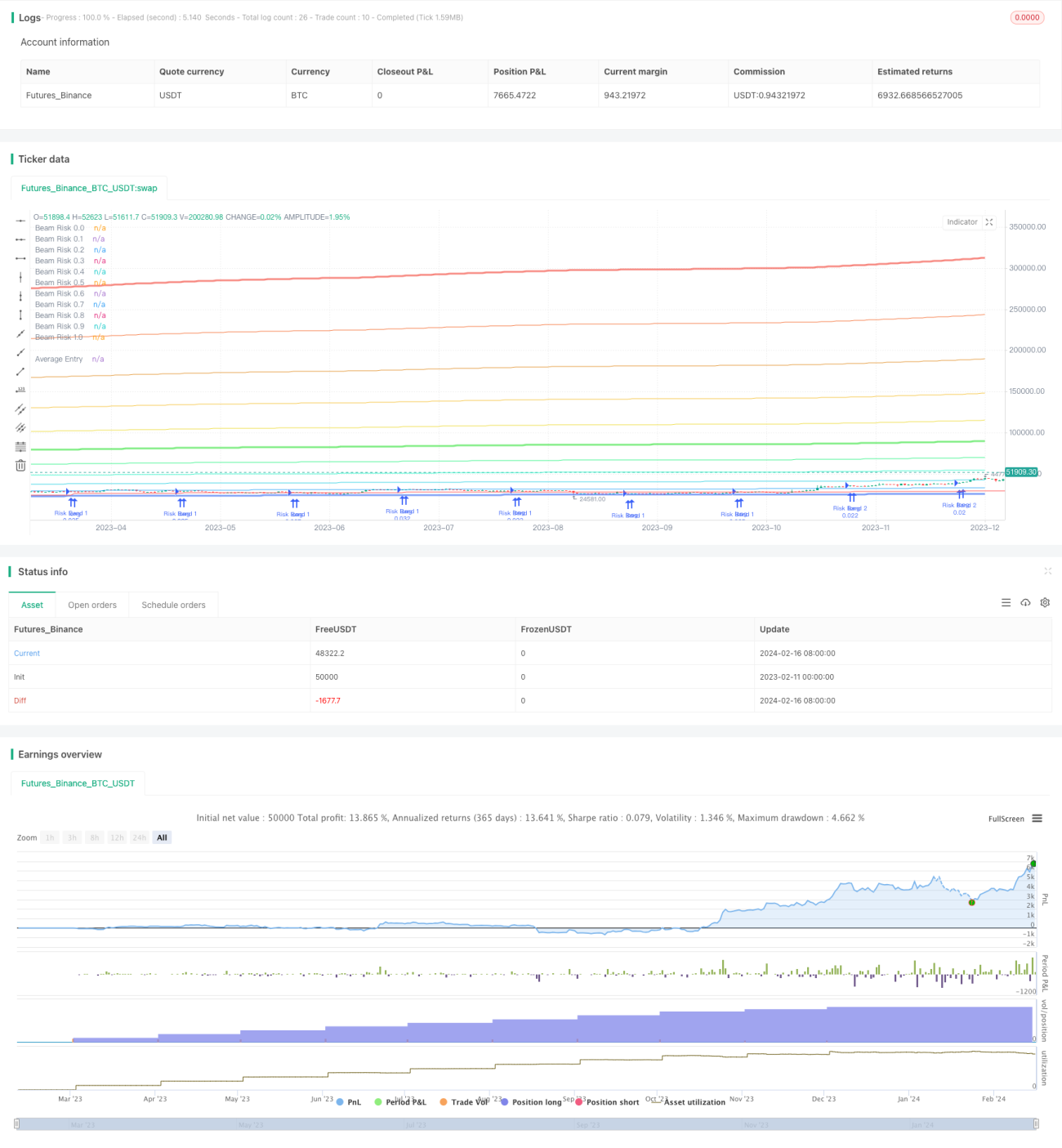
/*backtest
start: 2023-02-11 00:00:00
end: 2024-02-17 00:00:00
period: 1d
basePeriod: 1h
exchanges: [{"eid":"Futures_Binance","currency":"BTC_USDT"}]
*/
// © gjfsdrtytru - BEAM DCA Strategy {
// Based on Ben Cowen's risk level strategy, this aims to copy that method but with BEAM band levels.
// Upper BEAM level is derived from ln(price/200W MA)/2.5, while the 200W MA is the floor price. This is our 0-1 range.
// Buy limit orders are set at the < 0.5 levels and sell orders are set at the > 0.5 level.
//@version=5
strategy(
title = "BEAM DCA Strategy Monthly",
shorttitle = "BEAM DCA M",
overlay = true,
pyramiding = 500,
default_qty_type = strategy.percent_of_equity,
default_qty_value = 0,
initial_capital = 0) //}
// Inputs { ————————————————————————————————————————————————————————————————————
T_ceiling = input.string("Off", "Diminishing Returns", ["Off","Linear","Parabolic"], "Account for diminishing returns as time increases")
day = input.int(1, "DCA Day of Month",1,28,1,"Select day of month for buy orders.")
DCAamount = input.int(1000,"DCA Amount",400,tooltip="Enter the maximum amount you'd be willing to DCA for any given month.")
T_buy = input(true,"Buy Orders","Toggle buy orders.")
T_sell = input(true,"Sell Orders","Toggle sell orders.")
// Time period
testStartYear = input.int(2018, title="Backtest Start Year", minval=2010,maxval=2100,group="Backtest Period")
testStartMonth = input.int(1, title="Backtest Start Month", minval=1, maxval=12, group="Backtest Period")
testStartDay = input.int(1, title="Backtest Start Day", minval=1, maxval=31, group="Backtest Period")
testPeriodLen = input.int(9999, title="Backtest Period (days)", minval=1, group="Backtest Period",tooltip="Days until strategy ends") * 86400000 // convert days into UNIX time
testPeriodStart = timestamp(testStartYear,testStartMonth,testStartDay,0,0)
testPeriodStop = testPeriodStart + testPeriodLen
testPeriod() => true
// ——————————————————————————————————————————————————————————————————————————— }
// Diminishing Returns { ———————————————————————————————————————————————————————
x = bar_index + 1
assetDivisor= 2.5
switch
T_ceiling == "Linear" => assetDivisor:= 3.50542 - 0.000277696 * x
T_ceiling == "Parabolic"=> assetDivisor:= -0.0000001058992338 * math.pow(x,2) + 0.000120729 * x + 3.1982
// ——————————————————————————————————————————————————————————————————————————— }
// Risk Levels { ———————————————————————————————————————————————————————————————
cycleLen = 1400
getMaLen() =>
if bar_index < cycleLen
bar_index + 1
else
cycleLen
// Define Risk Bands
price = close
riskLow = ta.sma(price,getMaLen())
risk1 = riskLow * math.exp((assetDivisor)*0.1)
risk2 = riskLow * math.exp((assetDivisor)*0.2)
risk3 = riskLow * math.exp((assetDivisor)*0.3)
risk4 = riskLow * math.exp((assetDivisor)*0.4)
risk5 = riskLow * math.exp((assetDivisor)*0.5)
risk6 = riskLow * math.exp((assetDivisor)*0.6)
risk7 = riskLow * math.exp((assetDivisor)*0.7)
risk8 = riskLow * math.exp((assetDivisor)*0.8)
risk9 = riskLow * math.exp((assetDivisor)*0.9)
riskHigh = riskLow * math.exp((assetDivisor))
// Plot Risk Bands
p_low = plot(riskLow, "Beam Risk 0.0",color.new(#0042F0,50),3,editable=false)
p_band1 = plot(risk1, "Beam Risk 0.1",color.new(#0090F5,20),1,editable=false)
p_band2 = plot(risk2, "Beam Risk 0.2",color.new(#00C6DB,20),1,editable=false)
p_band3 = plot(risk3, "Beam Risk 0.3",color.new(#00F5BD,20),1,editable=false)
p_band4 = plot(risk4, "Beam Risk 0.4",color.new(#00F069,20),1,editable=false)
p_band5 = plot(risk5, "Beam Risk 0.5",color.new(#00DB08,50),3,editable=false)
p_band6 = plot(risk6, "Beam Risk 0.6",color.new(#E8D20C,20),1,editable=false)
p_band7 = plot(risk7, "Beam Risk 0.7",color.new(#F2B40C,20),1,editable=false)
p_band8 = plot(risk8, "Beam Risk 0.8",color.new(#DC7A00,20),1,editable=false)
p_band9 = plot(risk9, "Beam Risk 0.9",color.new(#F2520C,20),1,editable=false)
p_band10 = plot(riskHigh, "Beam Risk 1.0",color.new(#F01102,50),3,editable=false)
// ——————————————————————————————————————————————————————————————————————————— }
// Order Execution { ———————————————————————————————————————————————————————————
band5 = price<risk5 and price>risk4
band4 = price<risk4 and price>risk3
band3 = price<risk3 and price>risk2
band2 = price<risk2 and price>risk1
band1 = price<risk1
// DCA buy order weights
y = DCAamount / 5
switch
band5 => y:= y * 1
band4 => y:= y * 2
band3 => y:= y * 3
band2 => y:= y * 4
band1 => y:= y * 5
// Contracts per order
contracts =(y/price)
if testPeriod()
// Buy orders
if T_buy == true
if dayofmonth == day
strategy.entry("Risk Band 5",strategy.long,qty=contracts,when=band5)
strategy.entry("Risk Band 4",strategy.long,qty=contracts,when=band4)
strategy.entry("Risk Band 3",strategy.long,qty=contracts,when=band3)
strategy.entry("Risk Band 2",strategy.long,qty=contracts,when=band2)
strategy.entry("Risk Band 1",strategy.long,qty=contracts,when=band1)
// Sell orders
if T_sell == true
if strategy.opentrades > 5
strategy.exit("Risk Band 6",qty_percent=6.67,limit=risk6)
strategy.exit("Risk Band 7",qty_percent=14.28,limit=risk7)
strategy.exit("Risk Band 8",qty_percent=25.00,limit=risk8)
strategy.exit("Risk Band 9",qty_percent=44.44,limit=risk9)
strategy.exit("Risk Band 10",qty_percent=100,limit=riskHigh)
// ——————————————————————————————————————————————————————————————————————————— }
// Info { ——————————————————————————————————————————————————————————————————————
// Line plot of avg. entry price
plot(strategy.position_size > 0 ? strategy.position_avg_price : na,"Average Entry",color.red,trackprice=true,editable=false)
// Unrealised PNL
uPNL = price/strategy.position_avg_price
// Realised PNL
realPNL = 0.
for i = 0 to strategy.closedtrades-1
realPNL += strategy.closedtrades.profit(i)
// Size of open position in ($)
openPosSize = 0.
for i = 0 to strategy.opentrades-1
openPosSize += strategy.opentrades.size(i) * strategy.position_avg_price
// Size of closed position in ($)
closePosSize = 0.
if strategy.closedtrades > 0
for i = 0 to strategy.closedtrades-1
closePosSize += strategy.closedtrades.size(i) * strategy.closedtrades.entry_price(i)
invested = openPosSize+closePosSize // Total capital ($) put into strategy
equity = openPosSize+closePosSize+strategy.openprofit+realPNL // Total current equity ($) in strategy (counting realised PNL)
ROI = (equity-invested) / invested * 100 // ROI of strategy (compare capital invested to excess return)
// // Info Table
// var table table1 = table.new(position.bottom_right,2,9,color.black,color.gray,1,color.gray,2)
// table.cell(table1,0,0,"Capital Invested", text_color=color.white,text_halign=text.align_right)
// table.cell(table1,0,1,"Open Position", text_color=color.white,text_halign=text.align_right)
// table.cell(table1,0,2,"Average Entry", text_color=color.white,text_halign=text.align_right)
// table.cell(table1,0,3,"Last Price", text_color=color.white,text_halign=text.align_right)
// table.cell(table1,0,4,"Open PNL (%)", text_color=color.white,text_halign=text.align_right)
// table.cell(table1,0,5,"Open PNL ($)", text_color=color.white,text_halign=text.align_right)
// table.cell(table1,0,6,"Realised PNL ($)", text_color=color.white,text_halign=text.align_right)
// table.cell(table1,0,7,"Total Equity", text_color=color.white,text_halign=text.align_right)
// table.cell(table1,0,8,"Strategy ROI", text_color=color.white,text_halign=text.align_right)
// table.cell(table1,1,0,"$" + str.tostring(invested, "#,###.00"), text_halign=text.align_right,text_color = color.white)
// table.cell(table1,1,1,"$" + str.tostring(openPosSize, "#,###.00"), text_halign=text.align_right,text_color = color.white)
// table.cell(table1,1,2,"$" + str.tostring(strategy.position_avg_price, "#,###.00"), text_halign=text.align_right,text_color = color.white)
// table.cell(table1,1,3,"$" + str.tostring(price, "#,###.00"), text_halign=text.align_right,text_color = color.white)
// table.cell(table1,1,4, str.tostring((uPNL-1)*100, "#,###.00") + "%",text_halign=text.align_right,text_color = uPNL > 1 ? color.lime : color.red)
// table.cell(table1,1,5,"$" + str.tostring(strategy.openprofit, "#,###.00"), text_halign=text.align_right,text_color = uPNL > 1 ? color.lime : color.red)
// table.cell(table1,1,6,"$" + str.tostring(realPNL, "#,###.00"), text_halign=text.align_right,text_color = color.white)
// table.cell(table1,1,7,"$" + str.tostring(equity, "#,###.00"), text_halign=text.align_right,text_color = color.white)
// table.cell(table1,1,8, str.tostring(ROI, "#,###.00") + "%",text_halign=text.align_right,text_color = ROI > 1 ? color.lime : color.red)
// // ——————————————————————————————————————————————————————————————————————————— }