Stratégie d'indicateur technique des bandes de Bollinger basée sur la décomposition des séries chronologiques et la pondération du volume

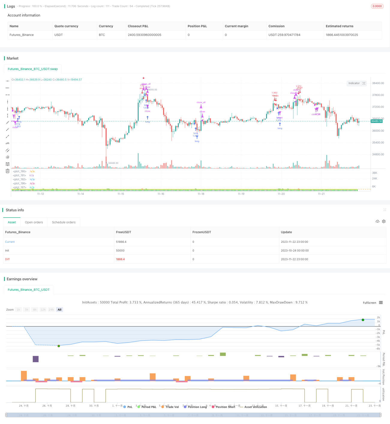
/*backtest
start: 2023-10-24 00:00:00
end: 2023-11-23 00:00:00
period: 1h
basePeriod: 15m
exchanges: [{"eid":"Futures_Binance","currency":"BTC_USDT"}]
*/

// This source code is subject to the terms of the Mozilla Public License 2.0 at https://mozilla.org/MPL/2.0/
//// This source code is subject to the terms of the Mozilla Public License 2.0 at https://mozilla.org/MPL/2.0/
// © oakwhiz and tathal

//@version=4
strategy("BBPBΔ(OBV-PVT)BB", default_qty_type=strategy.percent_of_equity, default_qty_value=100)

startDate = input(title="Start Date", type=input.integer,
     defval=1, minval=1, maxval=31)
startMonth = input(title="Start Month", type=input.integer,
     defval=1, minval=1, maxval=12)
startYear = input(title="Start Year", type=input.integer,
     defval=2010, minval=1800, maxval=2100)

endDate = input(title="End Date", type=input.integer,
     defval=31, minval=1, maxval=31)
endMonth = input(title="End Month", type=input.integer,
     defval=12, minval=1, maxval=12)
endYear = input(title="End Year", type=input.integer,
     defval=2021, minval=1800, maxval=2100)

// Normalize Function
normalize(_src, _min, _max) =>
    // Normalizes series with unknown min/max using historical min/max.
    // _src      : series to rescale.
    // _min, _min: min/max values of rescaled series.
    var _historicMin =  10e10
    var _historicMax = -10e10
    _historicMin := min(nz(_src, _historicMin), _historicMin)
    _historicMax := max(nz(_src, _historicMax), _historicMax)
    _min + (_max - _min) * (_src - _historicMin) / max(_historicMax - _historicMin, 10e-10)
    

// STEP 2:
// Look if the close time of the current bar
// falls inside the date range
inDateRange = true
     
     
// Stop loss & Take Profit Section     
sl_inp = input(2.0, title='Stop Loss %')/100
tp_inp = input(4.0, title='Take Profit %')/100
 
stop_level = strategy.position_avg_price * (1 - sl_inp)
take_level = strategy.position_avg_price * (1 + tp_inp)

icreturn = false
innercandle = if (high < high[1]) and (low > low[1])
    icreturn := true

src = close

float change_src = change(src)
float i_obv = cum(change_src > 0 ? volume : change_src < 0 ? -volume : 0*volume)
float i_pvt = pvt

float result = change(i_obv - i_pvt)

float nresult = ema(normalize(result, -1, 1), 20)



length = input(20, minval=1)
mult = input(2.0, minval=0.001, maxval=50, title="StdDev")
basis = ema(nresult, length)
dev = mult * stdev(nresult, length)
upper = basis + dev
lower = basis - dev
bbr = (nresult - lower)/(upper - lower)



////////////////INPUTS///////////////////
lambda = input(defval = 1000, type = input.float, title = "Smoothing Factor (Lambda)", minval = 1)
leng = input(defval = 100, type = input.integer, title = "Filter Length", minval = 1)
srcc = close

///////////Construct Arrays///////////////
a = array.new_float(leng, 0.0) 
b = array.new_float(leng, 0.0)
c = array.new_float(leng, 0.0)
d = array.new_float(leng, 0.0)
e = array.new_float(leng, 0.0)
f = array.new_float(leng, 0.0)

/////////Initialize the Values///////////
//for more details visit:
//          https://asmquantmacro.com/2015/06/25/hodrick-prescott-filter-in-excel/

ll1 = leng-1
ll2 = leng-2

for i = 0 to ll1
    array.set(a,i, lambda*(-4))
    array.set(b,i, src[i])
    array.set(c,i, lambda*(-4))
    array.set(d,i, lambda*6 + 1)
    array.set(e,i, lambda)
    array.set(f,i, lambda)

array.set(d, 0,  lambda + 1.0)
array.set(d, ll1, lambda + 1.0)
array.set(d, 1,  lambda * 5.0 + 1.0)
array.set(d, ll2, lambda * 5.0 + 1.0)

array.set(c, 0 , lambda * (-2.0))
array.set(c, ll2, lambda * (-2.0))

array.set(a, 0 , lambda * (-2.0))
array.set(a, ll2, lambda * (-2.0))

//////////////Solve the optimization issue/////////////////////
float r = array.get(a, 0)
float s = array.get(a, 1)
float t = array.get(e, 0)
float xmult = 0.0

for i = 1 to ll2
    xmult := r / array.get(d, i-1) 
    array.set(d, i, array.get(d, i) - xmult * array.get(c, i-1))
    array.set(c, i, array.get(c, i) - xmult * array.get(f, i-1))
    array.set(b, i, array.get(b, i) - xmult * array.get(b, i-1))

    xmult := t / array.get(d, i-1)
    r     := s - xmult*array.get(c, i-1)
    array.set(d, i+1, array.get(d, i+1) - xmult * array.get(f, i-1))
    array.set(b, i+1, array.get(b, i+1) - xmult * array.get(b, i-1))
    
    s     := array.get(a, i+1)
    t     := array.get(e, i)

xmult := r / array.get(d, ll2)
array.set(d, ll1, array.get(d, ll1) - xmult * array.get(c, ll2))

x = array.new_float(leng, 0) 
array.set(x, ll1, (array.get(b, ll1) - xmult * array.get(b, ll2)) / array.get(d, ll1))
array.set(x, ll2, (array.get(b, ll2) - array.get(c, ll2) * array.get(x, ll1)) / array.get(d, ll2))

for j = 0 to leng-3
    i = leng-3 - j
    array.set(x, i, (array.get(b,i) - array.get(f,i)*array.get(x,i+2) - array.get(c,i)*array.get(x,i+1)) / array.get(d, i))



//////////////Construct the output///////////////////
o5 = array.get(x,0)

////////////////////Plottingd///////////////////////



TimeFrame = input('1', type=input.resolution)
start = security(syminfo.tickerid, TimeFrame, time)

//------------------------------------------------
newSession = iff(change(start), 1, 0)
//------------------------------------------------
vwapsum = 0.0
vwapsum := iff(newSession, o5*volume, vwapsum[1]+o5*volume)
volumesum = 0.0
volumesum := iff(newSession, volume, volumesum[1]+volume)
v2sum = 0.0
v2sum := iff(newSession, volume*o5*o5, v2sum[1]+volume*o5*o5)
myvwap = vwapsum/volumesum
dev2 = sqrt(max(v2sum/volumesum - myvwap*myvwap, 0))
Coloring=close>myvwap?color.green:color.red
av=myvwap
showBcol = input(false, type=input.bool, title="Show barcolors")
showPrevVWAP = input(false, type=input.bool, title="Show previous VWAP close")
prevwap = 0.0
prevwap := iff(newSession, myvwap[1], prevwap[1])
nprevwap= normalize(prevwap, 0, 1)

l1= input(20, minval=1)
src2 = close
mult1 = input(2.0, minval=0.001, maxval=50, title="StdDev")
basis1 = sma(src2, l1)
dev1 = mult1 * stdev(src2, l1)
upper1 = basis1 + dev1
lower1 = basis1 - dev1
bbr1 = (src - lower1)/(upper1 - lower1)

az = plot(bbr, "Δ(OBV-PVT)", color.rgb(0,153,0,0), style=plot.style_columns)
bz = plot(bbr1, "BB%B", color.rgb(0,125,125,50), style=plot.style_columns)
fill(az, bz, color=color.white)



deltabbr = bbr1 - bbr
oneline = hline(1)
twoline = hline(1.2)
zline = hline(0)
xx = input(.3)
yy = input(.7)
zz = input(-1)
xxx = hline(xx)
yyy = hline(yy)
zzz = hline(zz)
fill(oneline, twoline, color=color.red, title="Sell Zone")
fill(yyy, oneline, color=color.orange, title="Slightly Overbought")
fill(yyy, zline, color=color.white, title="DO NOTHING ZONE")
fill(zzz, zline, color=color.green, title="GO LONG ZONE")

l20 = crossover(deltabbr, 0)
l30 = crossunder(deltabbr, 0)
l40 = crossover(o5, 0)
l50 = crossunder(o5, 0)


z1 = bbr1 >= 1
z2 = bbr1 < 1 and bbr1 >= .7
z3 = bbr1 < .7 and bbr1 >= .3
z4 = bbr1 < .3 and bbr1 >= 0
z5 = bbr1 < 0
a1 = bbr >= 1
a2 = bbr < 1 and bbr >= .7

a4 = bbr < .3 and bbr >= 0
a5 = bbr < 0
b4 = deltabbr < .3 and deltabbr >= 0
b5 = deltabbr < 0
c4 = o5 < .3 and o5 >= 0
c5 = o5 < 0
b1 = deltabbr >= 1
b2 = deltabbr < 1 and o5 >= .7
c1 = o5 >= 1
c2 = o5 < 1 and o5 >= .7

///

n = input(16,"Period")
H = highest(hl2,n)
L = lowest(hl2,n)
hi = H[1]
lo = L[1]
up = high>hi
dn = low<lo
lowerbbh = lowest(10)[1]
bbh = (low == open ?  open < lowerbbh ? open < close ? close > ((high[1] - low[1]) / 2) + low[1] :na  : na : na)




plot(normalize(av,-1,1), linewidth=2, title="Trendline", color=color.yellow)


long5 = close < av and av[0] > av[1]
sell5 = close > av

cancel = false
if open >= high[1]
    cancel = true


long = (long5 or z5 or a5) and (icreturn or bbh or up)
sell = ((z1 or a1) or (l40 and l20)) and (icreturn or dn) and (c1 or b1)
short = ((z1 or z2 or a1 or sell5) and (l40 or l20)) and icreturn
buy= (z5 or z4 or a5 or long5) and (icreturn or dn)


plotshape(long and not sell ? -0.5 : na, title="Long", location=location.absolute, style=shape.circle, size=size.tiny, color=color.green, transp=0)
plotshape(short and not sell? 1 : na, title="Short", location=location.absolute, style=shape.circle, size=size.tiny, color=color.red, transp=0)




if (inDateRange)
    strategy.entry("long", true, when = long )

if (inDateRange) and (strategy.position_size > 0)
    strategy.close_all(when = sell or cancel)
    

if (inDateRange)
    strategy.entry("short", false, when = short )

if (inDateRange) and (strategy.position_size < 0)
    strategy.close_all(when = buy)