Stratégie de moyenne des coûts du BTCdollar basée sur la bande BEAM

Aperçu
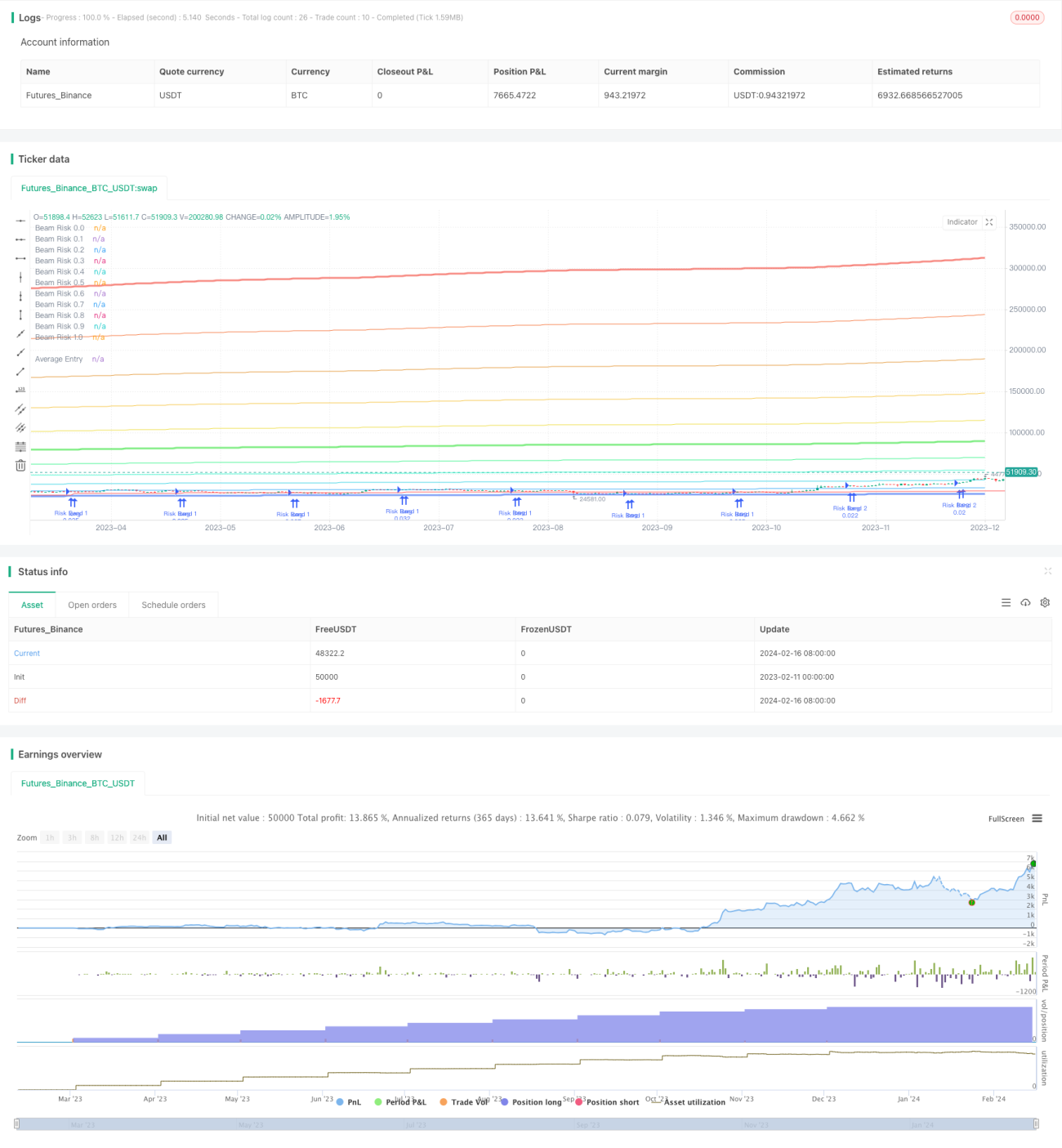
Cette stratégie, basée sur la théorie des niveaux de risque de Ben Cowen, vise à utiliser les niveaux de la bande BEAM pour réaliser une approche similaire. La limite supérieure de la bande BEAM est la moyenne mobile à 200 semaines après la prise de l'analogie, et la limite inférieure est la moyenne mobile à 200 semaines elle-même. Cela nous donne une portée de 0 à 1.
Principe de stratégie
La stratégie s'appuie principalement sur la théorie des bandes BEAM de Ben Cowen. Selon les variations de prix de la BTC, le prix peut être divisé en 10 zones comprises entre 0 et 1, qui représentent 10 niveaux de risque différents. Le niveau 0 représente le prix proche de la moyenne mobile sur 200 semaines, le moins risqué; le niveau 5 représente le prix dans la zone moyenne; le niveau 10 représente le prix proche de la trajectoire, le plus risqué.
La stratégie augmente progressivement la position d'achat lorsque le prix descend à un niveau bas. Plus précisément, si le prix se trouve dans la plage 0 à 0,5, un ordre d'achat est émis un jour du mois spécifié par la stratégie, et le montant de l'achat augmente progressivement avec la diminution du nombre de la plage. Par exemple, pour la vague 5, l'achat est de 20% du total des DCA du mois; pour la vague 1, l'achat est augmenté à 100% du total des DCA du mois.
Cette stratégie consiste à réduire progressivement la position lorsque le prix atteint un niveau élevé. En particulier, si le prix dépasse 0,5 bandes, un ordre de vente proportionnel est émis, et la position vendue augmente progressivement avec l'augmentation du nombre de bandes. Par exemple, lorsque la bande 6 est vendue à 6,67%; lorsque la bande 10 est vendue, toutes les positions sont vendues.
Analyse des avantages
Le plus grand avantage de cette stratégie de coût moyen de la DCA sur les ondes BEAM est qu'elle exploite pleinement les caractéristiques des transactions sur la volatilité de la BTC, en déposant des fonds lorsque le prix de la BTC tombe à des basses et en tirant des bénéfices lorsque le prix grimpe à des sommets. Cette pratique ne manque aucune opportunité d'achat ou de vente. Les avantages spécifiques peuvent être résumés comme suit:
- L'utilisation de la théorie BEAM pour évaluer les sous-évaluations des actifs et éviter les risques scientifiques;
- L'objectif est d'utiliser les caractéristiques de volatilité de la BTC pour saisir les meilleures opportunités d'achat et de vente avec une précision inégalée.
- L'adoption d'une approche de la moyenne des coûts permettant de contrôler efficacement les coûts d'investissement et d'obtenir des rendements stables à long terme;
- L'exécution automatique des transactions de vente et d'achat, sans intervention humaine, réduit le risque opérationnel;
- Paramètres personnalisables, stratégie d'adaptation flexible pour s'adapter aux changements du marché.
Dans l'ensemble, il s'agit d'une stratégie de régulation de paramètres sophistiquée qui permet d'obtenir des gains stables à long terme dans des conditions de volatilité de la BTC.
Analyse des risques
Bien que la stratégie BEAM Band DCA présente de nombreux avantages, il existe des risques potentiels à surveiller. Les principaux risques peuvent être résumés comme suit:
- La théorie et les paramètres de BEAM reposent sur des jugements subjectifs, avec une probabilité d'erreur;
- La tendance de la BTC est difficile à prédire et il y a un risque de pertes et de pertes.
- Les transactions automatisées sont vulnérables aux défaillances du système et au piratage de paramètres.
- Une fluctuation excessive peut entraîner des pertes importantes.
Les mesures suivantes peuvent être prises pour réduire le risque:
- Optimiser la définition des paramètres pour améliorer la précision des jugements théoriques BEAM;
- réduire de manière appropriée la taille des positions et le montant des pertes ponctuelles;
- Augmentation de la redondance et de la tolérance aux erreurs et réduction des risques liés aux opérations automatisées;
- Il est important de définir un point de rupture pour éviter des pertes monétaires excessives.
Direction d'optimisation
Compte tenu de ces points de risque, la stratégie peut être optimisée principalement dans les domaines suivants:
- Optimiser les paramètres de la théorie BEAM: ajuster les paramètres de la méthode log, les cycles de rétroaction, etc., pour améliorer l'exactitude des jugements du modèle;
- Optimisation du contrôle des positions: ajustement du montant total des DCA mensuels, du pourcentage d'achat et de vente, etc., afin de maîtriser le risque de perte unique;
- L'ajout d'un module de sécurité pour les transactions automatisées: mise en place de serveurs redondants, traitement local, etc. pour améliorer la tolérance aux erreurs;
- Module de stop-loss supplémentaire: paramétrez un point de stop-loss raisonnable en fonction des fluctuations historiques pour contrôler efficacement les pertes.
Ces moyens permettent d'améliorer considérablement la stabilité et la sécurité de la stratégie.
Résumer
La stratégie de coût moyen DCA de la bande BEAM est une stratégie de quantification qui a une grande valeur de combat. Elle utilise avec succès la théorie BEAM pour guider les décisions de négociation et est complétée par un modèle de coût moyen pour contrôler les coûts d'achat. En même temps, elle fait attention à la gestion des risques et à la mise en place de points de rupture pour éviter l'expansion des pertes.
/*backtest
start: 2023-02-11 00:00:00
end: 2024-02-17 00:00:00
period: 1d
basePeriod: 1h
exchanges: [{"eid":"Futures_Binance","currency":"BTC_USDT"}]
*/

// © gjfsdrtytru - BEAM DCA Strategy {
// Based on Ben Cowen's risk level strategy, this aims to copy that method but with BEAM band levels.
// Upper BEAM level is derived from ln(price/200W MA)/2.5, while the 200W MA is the floor price. This is our 0-1 range.
// Buy limit orders are set at the < 0.5 levels and sell orders are set at the > 0.5 level.- 1